ASTAP,
the Astrometric STAcking Program ASTAP
Forum Documentation
Version
history Checklist
for solving
ASTAP,
the Astrometric STAcking Program ASTAP
Forum Documentation
Version
history Checklist
for solving 
astrometric (plate) solver, stacking of images, photometry and FITS viewer
NEWS:
- 2026.06.29 ASTAP solver improved for star poor images.
- 2026.05.01 For Linux GTK3 widget versions have been released. Please report any problem with the layout of buttons and input fields.
- ASTAP versions released between 2025.04.13 and 2025.04.28 suffer a from bug which could hamper solving. Replace by version 2025.05.21 or later.
Download installers:
| Operating system | Program installer | Very
large STAR database installer |
Large STAR database installer | Smaller STAR database installer | Photometry STAR database installer for B,V | Wide field STAR database installer | Large GALAXY database installer | VARIABLE star database installer |
| Window 64 bit | Program (v2026.07.16) or development version | D80 | D50 | D20 or D05 |
V50_v2026.04.10 or V05 |
G05
or W08 |
Hyperleda.exe
(5 million galaxies) |
Variable stars (v2025.12.22) Nova positions retrieval program |
| Window 32 bit | Program zipped | |||||||
| Windows 11, 64 bit arm processor | See development version for command line version | |||||||
| Linux 64 bit | Program
debian (v2026.07.16), Program.tar.gz Program qt5.tar.gz compiled for QT5 widget openSUSE and Fedora support Also development version Also available at "Debian unstable". Arch Linux pkg |
D80 (debian) D80 (zipped) |
D50 (debian) D50 (arch) D50 (zipped) |
D20
or D05 |
V50_(v2026.04.10) or V05 |
G05
or W08 |
hyperleda.deb or hyperleda.zip (5 million galaxies) |
Variable stars (v2025.12.22) |
| Linux 32 bit | Program debian (v2026.07.16) | |||||||
| Raspberry PI, 32 bit | Program (v2026.07.16) | |||||||
| Raspberry PI, 64 bit | Program
debian (v2026.07.16) Program.tar.gz Program qt5 .tar.gz compiled for QT5 widget Arch Linux pkg |
|||||||
| MacOS 64 bit for intel processors | Program
(v2026.07.16) OpenSSL 1.1 for internet access |
D80 | D50 To remove old database files, press in finder Command+Shift+G and go to /usr/local/opt/astap and select the old files and move them to Bin. |
D20
or D05 |
V50_v2026.04.10 or V05 |
G05
or W08 |
hyperleda.pkg (5 million galaxies update. The 2.1 million object version is included with the star database |
Variable stars (v2025.12.22) |
| MacOS 64 bit for Apple silicon processors (M-types) | Program (v2026.07.16)
code signing required! See instructions at this link (bottom)!!
Significant faster. (Dcraw and FITS
compression are not available in this version OpenSSL 1.1 for internet access |
You have to install:
2) One of the star databases.
You will need only one database. Is your field of view 0.6 degree or larger you can download either the D05 or D20 or D50 or D80. The D05 is the smallest. The D80 is the largest. Using the D80 has no drawback accept it is larger, about 1.25 gbyte. If you have one of the older H17, H18, V17 G17, G18 star databases, they can be uninstalled/deleted.
Star databases usability:
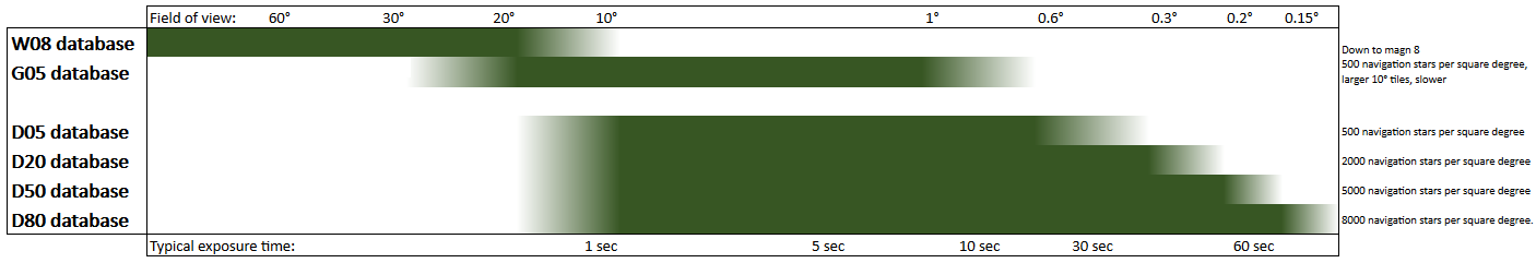
Instead of a magnitude limit the new databases have a density limit. These databases have been sorted on star density up 500, 2000, 5000 or 8000 stars per square degree. This should guarantee that in star-poor-areas there will be sufficient faint stars in the database for navigation (solving). In star-rich areas only a limited amount of bright stars is included keeping the star database size moderate. If required these databases will go as deep as magnitude 21.
This will be beneficial for setups with a small field-of view. There should be always enough database stars available for navigation.
The V50 photometry database has like the D50 a 5000 stars per square degree density except the magnitude is the calculated Johnson-V and it also contains the Gaia Bp-Rp magnitude difference. The V05 photometry database is like the G05 except the magnitude is the calculated Johnson-V and it also contains the Gaia Bp-Rp magnitude difference.
For comment feedback and questions there is the ASTAP Forum. The ASTAP Manual is below
For photometry you could download and install the V50 star database. It contains the calculated Johnson-V magnitude and colour information (GBp-GRp) for star annotations. This one also works best for solving an image with a FOV of more then ten degrees
Hyperleda, a very large galaxy database for deep sky annotation. 2.190.000 objects. Based on extract from leda.univ-lyon1.fr/ Will be placed in the program directory.
For Linux in case of OpenSSL error try this: sudo apt install libssl-dev
Alternative links & development version:
| Operating system | Program development version | Alternative
star database links |
Barebone command-line solver compatible with the GUI version if renamed. No pop-up notifier. Will not accept raw files and will not work with SharpCap since FOV is not stored. |
| Window 64 bit | ASTAP_installer_(v2026.07.13),
ASTAP executable only |
D80
zipped, I80 zipped (Cousins Ic), D50 installer, V50 zipped, D20 installer, D05 installer, G05 zipped, W08 zipped, H18 installer, (obsolete) H18 zipped, (obsolete) |
astap_cli (v2026.07.16 |
| Window 32 bit | ASTAP_zipped file | astap_cli (v2026.07.16 | |
| Window11 arm64 | astap_cli (v2026.07.16) On Windows arm 375% faster. Can be renamed from astap_cli.exe to astap.exe | ||
| Linux 64 bit | ASTAP_debian_package_(v2026.07.16),
ASTAP tar.gz ß version debian using GTK3 ß version tar using GTK3.tar.gz ß version Arch Linux GTK3 pkg |
D80
zipped, I80 zipped (Cousins Ic), D50 installer, V50 zipped, D20 installer, D05 installer, G05 zipped, W08 zipped, H18 installer (obsolete) H18 zipped, (obsolete) H18 debian(obsolete) H18 zipped (Obsolete) for manual install at /opt/astap V17 zipped (obsolete), |
astap_cli (v2026.07.16) |
| Linux 32 bit | ASTAP_debian_package_(v2026.07.16) | ||
| Raspberry PI, 32 bit | ASTAP_debian_package_(v2026.07.16) | astap_cli (v2026.07.16) | |
| Raspberry PI, 64 bit | ASTAP_debian_package_(v2026.07.16) ß version debian using GTK3 ß version tar using GTK3.tar.gz |
astap_cli (v2026.07.16) | |
| MacOS 64 bit | astap_mac_X86_64.zip
(v2026.06.29) Executable only. Move the executable in the application at /Contents/MacOS |
DD80
zipped, I80 zipped (Cousins Ic), D50 installer, V50 zipped, D20 installer, D05 installer, G05 zipped, W08 zipped, H18 installer, (obsolete) H18 zipped, (obsolete) |
astap_cli (v2026.07.16) |
| MacOS M1 | astap_mac_M1.zip
(v2026.06.29) Executable only. Move the executable in the application at /Contents/MacOS |
astap_cli (v2026.07.16) code signing required! | |
| Android arm 64 bit | Use a star database from above. | astap_cli
(v2026.07.16) zipped. Included in these third party apps OpenLiveStacker and in Stellar finder |
|
| Android arm 32 bit | astap_cli
(v2026.07.16) zipped. Included in this third party app OpenLiveStacker |
||
| Android X86_64 | astap_cli (v2026.07.16) zipped. No GUI application available. | ||
| Android X86 | astap_cli (v2026.07.16) zipped. No GUI application available. |
- Questions, feedback: ASTAP Forum
- Older versions are available at Sourceforge
- Version history
- Source code (Object Pascal, Lazarus/FPC)
-
- Introduction
- Program installation
- Program operation, stacking astronomical images
- Stack menu
- Lights tab
- Darks tab
- Flats tab
- Flat darks tab
- Results tab
- Stack method tab
- Stacking grayscale of colour stacking
- Stacking raw one shot colour images (OSC)
- RAW conversion of OSC images (one shot colour images)
- Stacking LRGB
- Image
stiching
- Alignment menu tab
- Blink tab
- Photometry tab
- Photometry
- The filter & database compatibility
- Testing
your photometric measurements
- Transformation
- Transformation
test
- Measure all visible variables in one step
- Measuring asteroid magnitudes
- Pop-up menu photometry tab
- Photometry using the command-line
- Inspector tab
- Mount analyse tab
- Live stacking
- Monitoring
- Pixel math tab 1 and 2
- Background equalization tool
- Popup menu
- Viewer:
- FITS thumbnail viewer
- Tools menu:
- Batch processing
- Image inspection
- F5 menu
- Curvature
and tilt indication
- HFD_2d_contour
- HFD_diagram
- Median_background_values
- HFD values
- Unroundness
of the imaged stars.
- Show
distortion
- Aberration
Inspector
- Photometry calibration
- SQM measurement
- Star annotation and photometry
- Asteroid annotation
- Deep sky annotation
- View menu
- Pop-up menu viewer
- Star info to clipboard.
- Online query.
- Gradient removal tool
- Dark spot removal tool
- Copy paste tool
- Remove deep sky object
- Remove borders
- Crop
fits image
- FITS tables
- Other
pop-up menus
- Solver, usage as astrometric solver and command line options
- Appendix 1 stack process
- Appendix 2 Why using flat-darks or bias
- Appendix 3 the star database 1476 and 001 format.
- Appendix 4 FITS keywords read for solving.
- Developer information: Using SIP Coefficients for optical distortion correction
- Background info, ASTAP star pattern recognition and astrometric (plate) solving algorithm.
- Background info, Reverse mapping in image stacking.
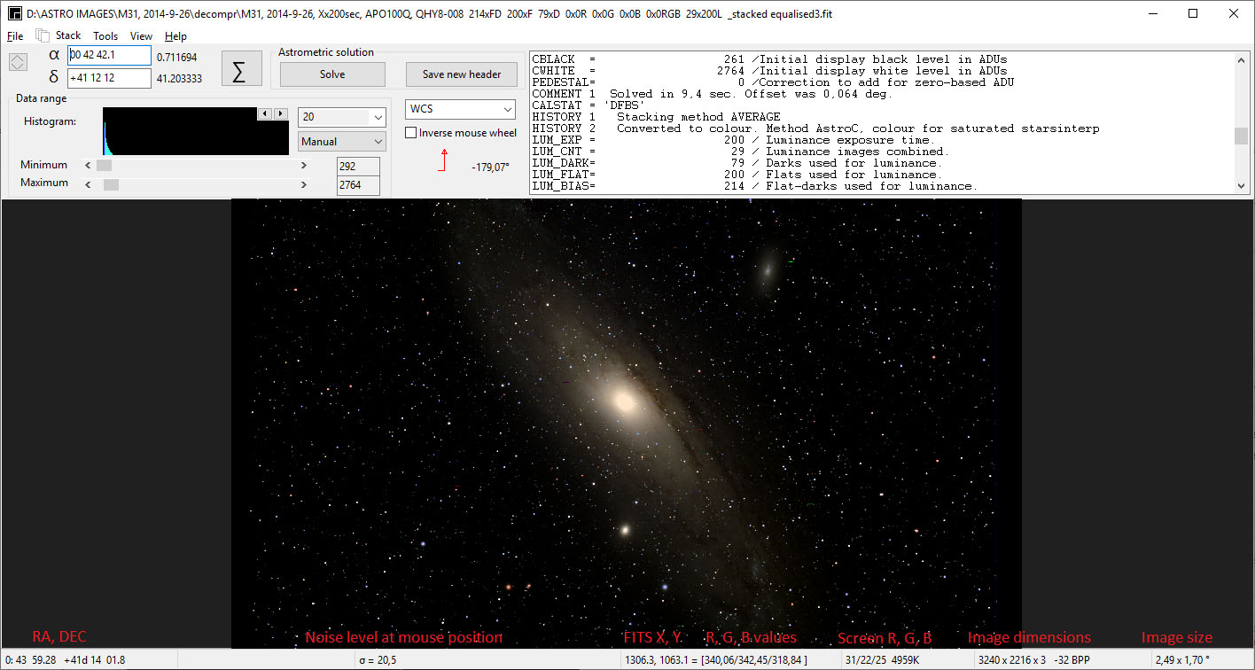
ASTAP is a free stacking and astrometric solver (plate solver) program for deep sky images. It works with astronomical images in the FITS format, but can import RAW DSLR images or XISF, PGM, PPM, TIF, PNG and JPG images. It has a powerful FITS viewer and the native astrometric solver can be used by CCDCiel, NINA, APT, Voyager or SGP imaging programs to synchronise the mount based on an image taken.
Main features:
- Stacking astronomical images including dark frame and flat field correction.
- Filtering of deep sky images based on HFD value and average value.
- Alignment using an internal star match routine, internal astrometric solver.
- Mosaic building covering large areas using the astrometric linear solution WCS or WCS+SIP polynomial.
- Background equalizing.
- FITS viewer with swipe functionality, deep sky and star annotation, photometry and CCD inspector.
- FITS thumbnail viewer.
- Results can be saved to 16 bit or float (-32) FITS files.
- Export to JPEG, PNG, TIFF( ASTRO-TIFF), PFM, PPM, PGM files.
- FITS header edit.
- FITS crop function.
- Automatic photometry calibration against Gaia database, Johnson -V or Gaia Bm
- CCD inspector
- Deepsky and Hyperleda annotation
- Solar object annotation using MPC ephemerides
- Read/writes
FITS binary and reads ASCII tables.
- Some pixel math functions and digital development process
- Can display images and tables from a multi-extension FITS.
- Blink tab.
- Track and Stack function
- Photometry tab
- Inspector tab for measuring curvature.
- Mount analyse tab.
- Live
stacking tab.
- Available for MS-Windows 32 & 64 bit, Linux 32, 64 bit, MacOS 64 bit, Raspberry-Pi Linux 32 and 64 bit.
Stacking of images:
Stacking of astronomical images is done to achieve a greater signal to noise ratio, prevent sensor saturation and correct the images for dark current and flat field. Additionally imperfect images due to guiding, focus problems, or clouds can be removed.
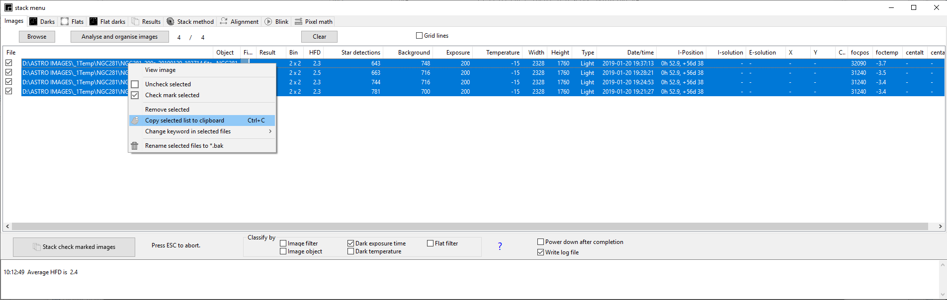
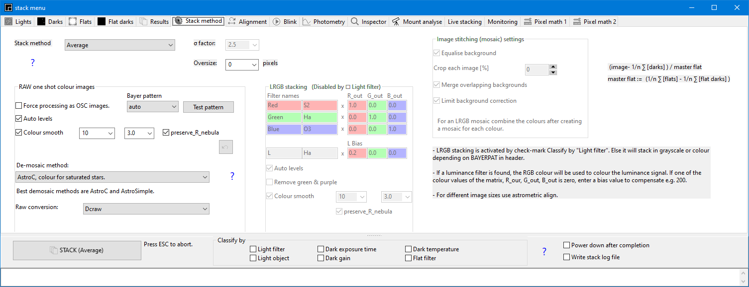
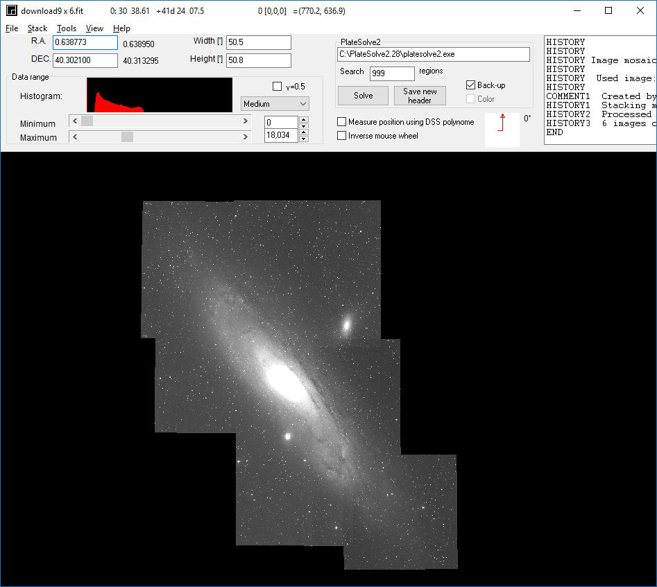
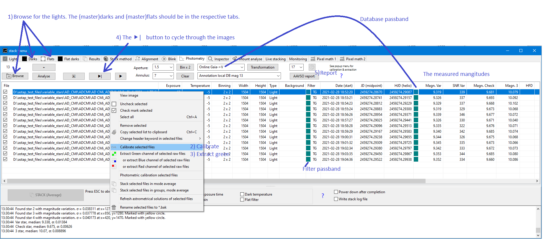
This is a screen short of the stack menu. It contains several tabs for the file list and settings. File can be sorted on quality and values.The image can be visually inspected in the viewer by a double click on the file or using the pop-up menu.
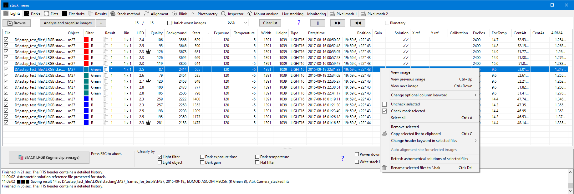
Program requires FITS images or RAW files as input for stacking, but it can also view 16 bit PGM /PPM files, XISF files or in 8 bit PNG, TIFF or BMP files. For importing DSLR raw images the program DCRAW from David Coffin or LibRaw is used.
- Stacking methods: average and sigma-clipping-average.. Internal calculation using floating point numbers. Latest program versions are using reverse mapping with bilinear interpolation.
- Simple and intuitive user interface.
- Automatic saving of selected options and files.
- Can create master files for dark and flat & flat-darks to reduce processing time.
- Limited memory use, independent of the number of images stacked.
- Bayer algorithm for DSLR/OSC cameras
Astrometric Solving:
ASTAP can be used as astrometric solver to synchronise the telescope mount position with centre position of an image taken with the telescope. Existing images can be solved to annotate, for photometry or the measure positions of unknown objects.
The ASTAP solver aims at a robust star pattern recognition using the catalog star coordinates in Equinox J2000. The solution is not corrected for optical distortion, refraction, proper motion of stars and other minor effects all to be very minor.
The process astrometric solving is often referred to as a "plate solve". That was a correct description in the past, but in modern times there are no photographic plates involved in the process.
Back to index
Program installation:
MS-Windows:
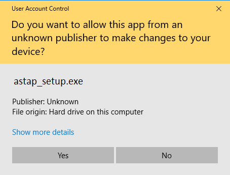
Note that for Windows ASTAP is seen as an unknown publisher. For Win10 you have to click trough the following screens.
Click on astap_setup.exe to install.
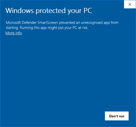
Click op "More info"
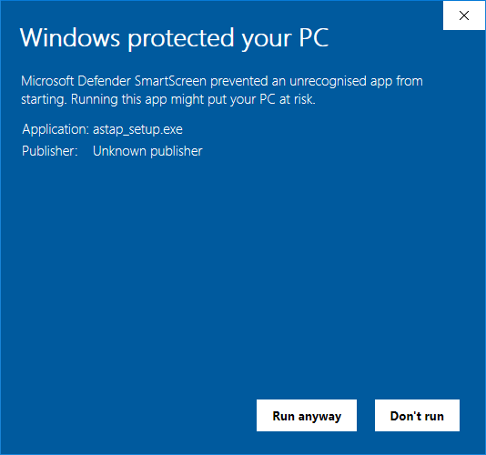
Click op "Run anyway"
Do the same for the database installer.
Linux installation:
MacOS installation:
The program and star databases are provided as pkg files. Download and right-click on the astap.pkg and select install. Same for the star database file.
On Sequoia 15.1, you can no longer right click on the package and override MacOS complaining about it being from an unknown developer. You'll need to go into System Settings->Privacy & Security and scroll to the bottom and select astap.pkg to allow installation
For Mac's with an M processor like the M1 do the following for code signing:
Open a terminal windows and copy paste and execute the following command:
codesign --force -s - /Applications/ASTAP.app/Contents/MacOS/astap
Note: The star database will be installed at /usr/local/opt/astap/
Program operation, stacking astronomical images:
The purpose of the stacking routine is to combine astronomical images to reduce noise and to flatten the image.
Ideally you should have collected
- 1a) Several light frames. Images of deep sky object unprocessed.
- 1b) Several dark frames of the same temperature and exposure as the light frames. A dark frame is a frame that represents an exposure duration done in total darkness. This signal includes the bias signal, but also includes any dark current charge accumulation, and thus any dark current noise that exists within the dark current signal. For a dark suburban area (SQM=20.4) you should take about the same amount or more darks as lights. For a light polluted area you could take less darks then lights since the noise in the lights generated by the sky background will be abundant.
- 2a) Several flat frames. A flat frame is a frame that represents the field flatness and taken from an uniform light source. Ideally with a significant signal level. This to compensate for vignetting and dust particles. Vignetting can greatly darken the corners of your image and have to be compensated.
- 2b) Flat dark frames or bias frames ideally taken of the same temperature and exposure duration as the flats. Since flats are taken with very short exposure times, either flat dark or bias images of almost zero seconds will do. See also why flat-darks
The automatic stacking process in ASTAP goes through the following steps:
- The flats will be combined to an average and the combined average flat-darks will be subtracted to have a near ideal presentation of the vignetting called the master flat frame.
- The darks will be combined to an average master dark.
- From each light frame, the master dark will be subtracted to extract the pure deep sky signal.
- Each light frame will be flattened by dividing it by the master-flat resulting in corrected light frames.
- The corrected light frames are combined to the final image using the average or sigma clip mean (to remove outliers as satellite tracks) method.
It is possible to mix different exposure times but it is not recommended for the frames of one colour. The reason is that sigma clipping of pixel value outliers could work less efficient for frames with different exposure times. The frames will be combined with a weight factor relative to the exposure time but the image noise will not be fully linear with the exposure time. E.g. the read noise is fixed. Once the individual colours are combined then the exposure times are no longer relevant.
So you could expose all red frames for 60 seconds and all green frames with 120 seconds and combine them. But combining red frames of 60 and 120 seconds is less desirable.
Operation of the stacking program
Start the ASTAP program.
Call up the stack menu window using the ∑ button.
a) Select frames
In the tab images, select the lights. In the tab dark, select the corresponding darks. In the tab flats, select the flat-field images called flats and in tab flats-darks the flat-darks/bias frames. In most cases you could select all frames in tab images. The program will move the fames to the corresponding tab during analyse. The lights and darks should preferably have the same exposure time and temperature. The flats should have the same exposure time and temperature as the flat-darks.
b) Analyse and remove bad frames
In the images tab (for the light frames), press analyse and remove manually any poor image. Poor images can be detected by a too high HFD (Half flux diameter stars), low number of stars or high background values (caused by clouds) . Loss of tracking could result in too low HFD value. If required inspect each image by double on the file name. The list can be sorted by clicking on the corresponding columns. Using the pop-up menu selected bad frames can be renamed to *.bak for deletion later.
c) Set parameters in tab stack method
In the tab stack method, select the stacking method, average or sigma-clip-average. For OSC camera images, select "Convert OSC images to colour". Select the correct Bayer pattern (4 options). Test the required pattern first in the viewer with an image. The source images should be raw (gray) without colour produced by astronomical camera's.
d) Set parameters in tab alignment
Leave this to the default star alignment.
e) Classify by
Leave all checkboxed initially unchecked. (This is an option to select automatically a master dark with the correct temperature and exposure time for the lights. Same for master flat selection based on filter used both in the light and flat.)
f) Press the Stack (..) button.
The darks and flats & flat-darks will be combined in a master dark and master flat frame. Then the program will combine the light frames to the final image and save it automatically to FITS. This will take some time.
g) Export
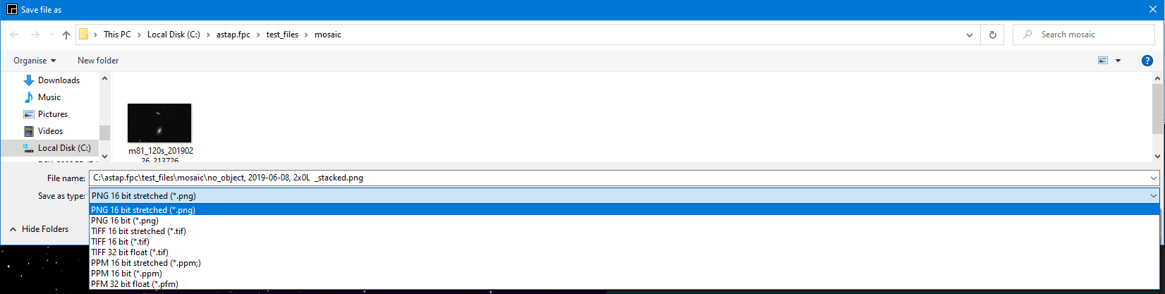
The stack result will be saved as a FITS file. The program keeps a record of all results in tab Results. Stretch the image as required. Crop the edges if required using the pop-up menu. Equalise the back ground if required using the tool in tab pixel math. Export as stretched JPG or 16 bit bit stretched/unstretched PNG / TIFF. The stretched export follows the gamma and stretch setting of the display. For further image processing you could export to 32 bit float TIFF or 32 bit float PFM format.
ASTAP export types:
| File formats ASTAP | 8 bit | 16 bit | 32 bit (float) |
| Import | FITS, JPEG, PNG, TIFF, XISF (uncompressed) | FITS, FITS.FZ, PNG, TIFF (ASTRO-TIFF), PPM, PGM, raw formats, XISF (uncompressed) | FITS, FITS.FZ, TIFF (ASTRO-TIFF), PFM,XISF (uncompressed) |
| Export | FITS, JPEG, PNG, TIFF | FITS, FITS.FZ, PNG, TIFF (ASTRO-TIFF), PPM, PGM | FITS, TIFF (ASTRO-TIFF), PFM |
From version 2026.07.16, ASTAP natively supports fits rice compressed files with extension fits.fz. GZIP compression is not supported.
All the program settings and file selections will be save d by leaving the program or click on the "Stack button".
Back to index
The stack menu:
For a generic description how to stack see Program operation, stacking astronomical images
Lights tab
Browse button: Images, darks, flats can be added using the Browse button or can be drag dropped on the form. You can also drag drop multiple directories on the stack tabs. Note it will included the files in any subdirectory or subsubdirectory. (v2025.01.16)
Analyse and organise button: Images placed in the first tab will be organised based on the FITS header keyword IMAGETYP. As soon as you click on the image Analyse and organise button, dark and flats and flat-darks/bias images will be moved to the corresponding tab. If the button is pressed are also the images are analysed for HFD, background and other details.
For LRGB stacking if a question mark in column "Filter" is displayed then filter name in the "Stack method tab" should made the same as in the flat header behind the keyword FILTER.
Check-mark the frames. Only check-marked frames are stacked. Light files names containing "_stacked" will be un-checked by default to prevent stacks by accident are re-used. If required, just select the file and check-mark it again.
Sorting: Images can be sorted by any of the columns. For example if you click on HFD, the images will be sorted on HFD. You could then remove the images with the highest values or inspect them by double -clicking on the file name.
Classify by:
- Light filter classification: If classify by light filter is check marked then the stack routine will combine the available filters to a RGB image. If only Red + Green +Blue image are available they will be combined in a RGB image. If Luminance images are available it will first stack the RGB colors and then apply a most-common-filter and Gaussian blur on the RGB result. Finally the luminance image is coloured with the RGB result. The filter factor should be set typically near 20. The filter names can be set in tab alignment
- Dark classification: The dark tab can contains multiple master darks. To select automatically the best compatible master set the check-mark for exposure and or temperature. If set the master dark with compatible exposure duration and or temperature is automatic selected. If more then one compatible dark is found then the dark with nearest date is selected. Master darks with incompatible dimensions are ignored.
- Flat filter classification: The flat tab can contains multiple master flat made with different filters. To select automatically the best compatible flat set the check-mark for classify flat on filter. Master flats with incompatible dimensions are ignored.
- Object
classification: Several image series of different objects
can be stacked in one run. If the classify-by-object is check-marked,
the program will stacked in groups based on the OBJECT header keyword
value.
| Classification-during-stacking | Object | Filters equal? | Dates equal? | Exposures equal? | Gains equal? | Temperatures equal? |
| Light | ✔ | ✔ | use nearest | ✔ | ✔ | ✔ |
| Dark | ||||||
| Flat | ✔ | warning (results-tab) | warning (results-tab) | warning (results-tab) | ||
| Flat-dark |
Lights tab, How to exclude poor images
Before stacking the images can be analysed with the Analyse and organise images button. Images can be sorted on any of the columns like 1) HFD value, 2) Quality, 3) Star detections or 4) background value. For example if you click on HFD, the images will be sorted by HFD. You could then remove the images with the highest value from the list or inspect them by double click on the file name. The poor quality images can be renamed to *.bak in bulk by the pop-up menu to be removed/deleted later. The renaming to *.bak can be undone by pressing CTRL+Z or META+Z for the Mac.
- HFD is the image median HFD. The lower the value, the better. The HFD value is depended on focus quality and guiding precision. Note that low values could be the result of streaks as a result of loss of tracking.
- Quality of the image. The higher, the better. Based on the number of star detections divided by HFD. Depending on sky transparency of the sky and focus. Note that loss of tracking could results in a low HFD and low star count so a low quality factor..
- Star level. The higher the better. Depending on transparency of the sky and focus. Note that a high values indicate satellite tracks.
- Background. Depending on sky darkness and transparency. The lower the better. A higher value means in most cases a cloud was blocking the sky.
- Sharpness. The lower the better.Measures the change between dark and bright pixels. The measurement is very sensitive to satellite tracks. Could be used to detect satellite track when compared with HFD value. Could also be used to sort images of the Moon and Sun on sharpness.(but they can't be stacked) For correct sharpness measurement of OSC images either the FITS header should contain the keyword BAYERPAT or check-mark "Convert OSC to colour" in tab "Stack method".
For a normal distribution you could expect the following:
| Confidence interval | Proportion within |
| 1σ | 68% |
| 1.5σ | 87% |
| 2σ | 95 % |
| 2.5σ | 98.8% |
| 3σ | 99.7% |
Lights tab, satellite tracks
The stack method "sigma clip average" should normally remove any satellite tracks. If after stacking with "sigma clip average" there are still satellite tracks visible, you could lower in tab "Stack Method". the sigma factor from 2.5 to a lower value maybe 2 or even 1.5 . An other way is the blink/scroll through the images with the >> button. As soon you see an abnormal bright track on the image stop the blinking by esc and inspect visually the image(s) involved by double click on the row. Remove any poor image by using right mouse button pop-up menu "rename to *.bak"
If the + option is used then additionally the number of detected satellite streaks will reported in a column. Frames with very bright tracks could be removed
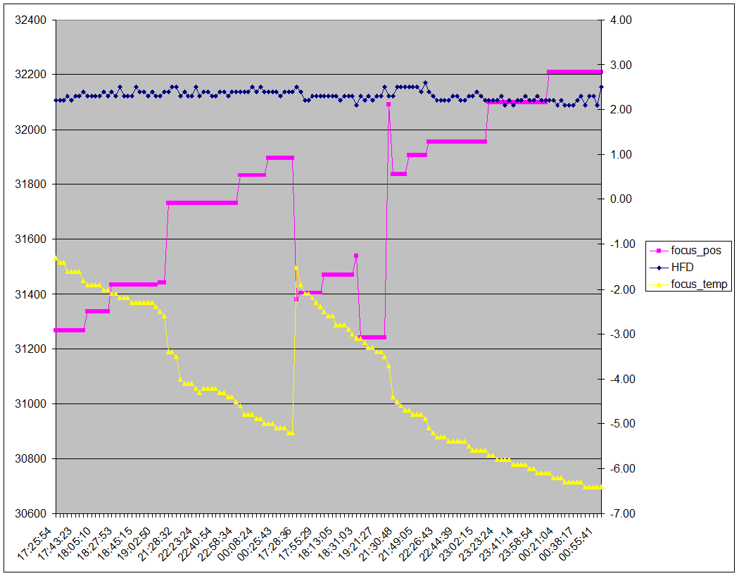
Configurable column
The last column in tab lights can report any image header value. To configure set in the pop-up menu the header keyword to read. This configurable option can be used to report e.g the measured SQM, TILT as written by the batch processing menu of the viewer.
Lights tab, Copy selected list to clipboard
This menu allows the export the
listed FITS data to a spreadsheet. Sselect
all relevant files and copy the data with right mouse button. Then copy
the data into a spreadsheet for analysis.
Here and example of the data analysed in a
spreadheet:
Back to index
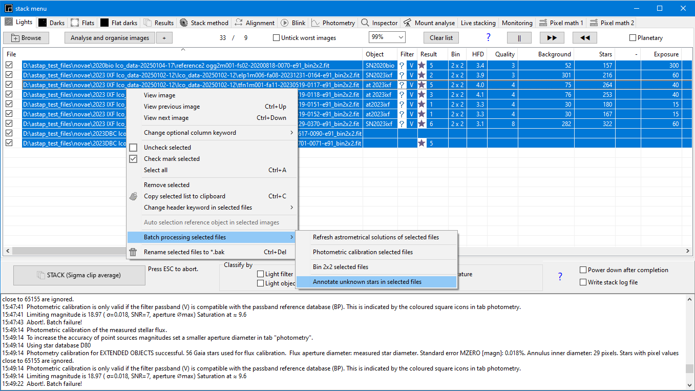
This popup menu of the tab lights will allow batch processing of the selected files and annotate any unknown stars. These could be a nova. The algorithm will annotate novae candidates by comparing star detection's with the online Gaia star catalogue. Any detected star which is missing in the catalgue is annotated. The number of detections is reported in column result.
The same algorithm is accessible from the viewer menu.
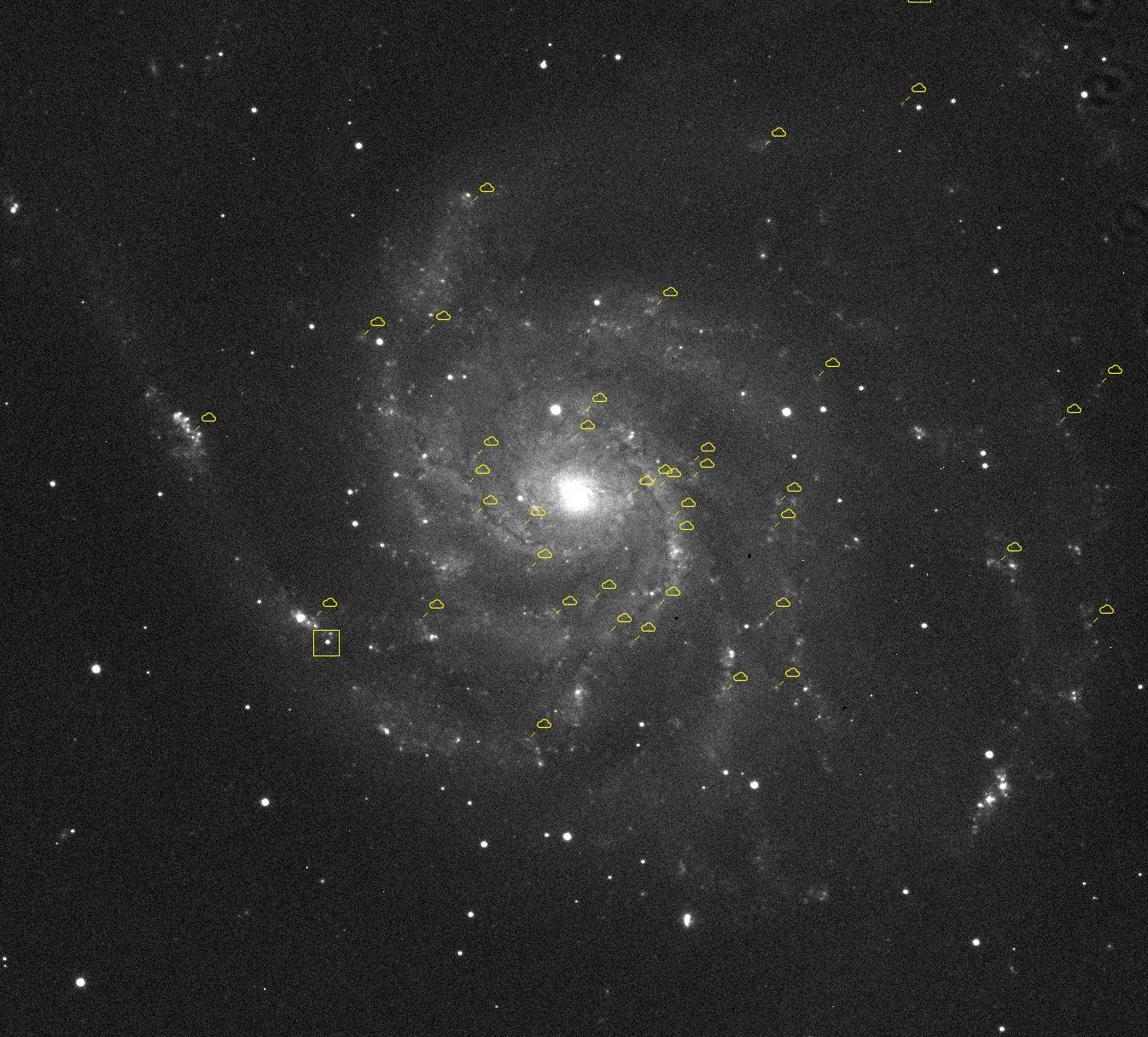
The image need to be sharp to differentiate between small galaxies and novae. Poor focussed or bad tracking will result in more false detections.
Below an example of a nova and non-star detection in M101
Database for novae
There is a small utility nova_positions_retrieval.zip for Windows to retrieve the nova positions from www.rochesterastronomy.org/supernova.html and writes it to the variable star database variable_stars_15.csv. Extract the utility program at the ASTAP directory or place the output file variable_stars_15.csv in the ASTAP directory. Select in the photometry tab for annotation "Local database mag 15". Select in the viewer "Variable star annotation", shortcut CTRL+K. If you need this utility for Linux or Mac tell me.
Lights tab, pop-up menu, change header keyword batch wise.
Change header keywords of selected files: The pop-up menu has an option to update a keyword in multiple files if required. Select the files to modify and select the pop-up menu with the right mouse button. If you type for the new keyword value in capital letters DELETE, then the keyword will be removed from all file headers.
If the keyword DATE-OBS is typed then the program will request a time shift in hours or a fraction of an hour. This could be used to correct a recorded time of observation. The old DATE-OBS value is stored behind a new keyword like TT120619 for recovery by renaming it back to DATE-OBS.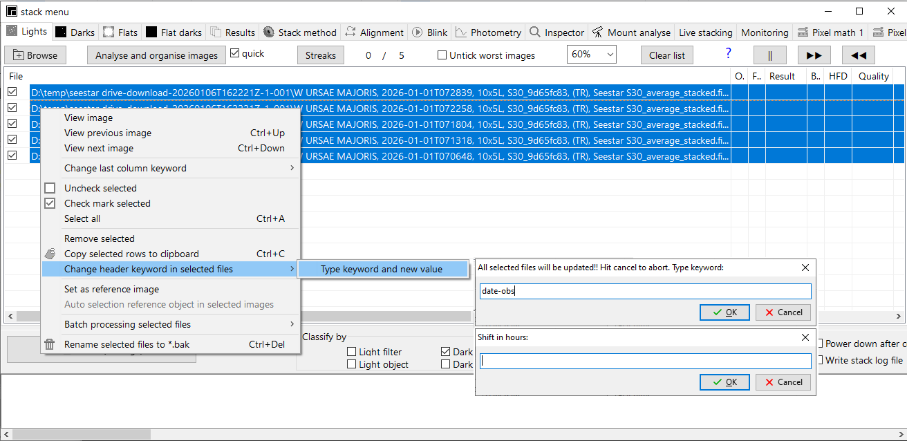
Darks tab:
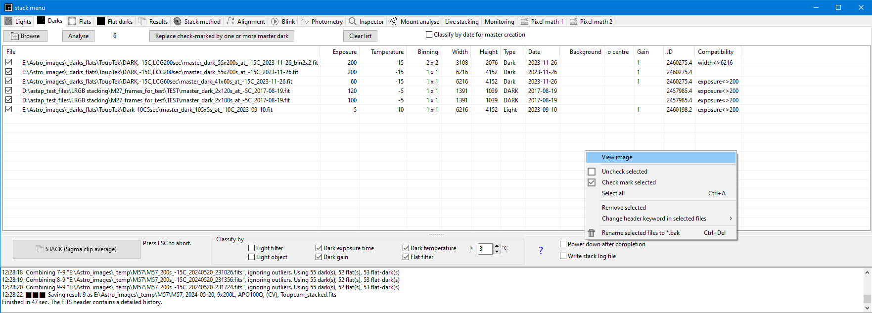
Browse button: use this button to add frames to the list. Frames can also be drag dropped on the form.
Replace check-marked by one or more master darks: This will replace the individual check-marked frames with a single master dark. The existing master darks will not be effected.
Classify during creation
If the list contains frames with different exposure durations and the option "classify by" exposure time is check-marked then for each exposure duration a different master dark will be created. Same applies for gain and temperature. If not classify check- marks are set then all loaded individual dark frames will be combined in one master dark and values are averaged. To automate making a master flat for each observation night you could use the Classify by date for master creation check mark at the top of the tab. This will create master flats for each exposure night from the frame loaded.
| Dark-classification-during-master-creation | filter | date | exposure | gain | temperature |
| Dark | ✔ | ✔ | ✔ | ✔ | ✔ |
Classify during stacking
The intention is to keep all master darks here loaded and check-marked. Master dark selection on light exposure, gain and temperature can be fully automatic by setting the "classify on" check-marks. If two master darks only differ in date then the frame with the date closest to the light will be selected. Closest date selection is intended for DSLR users without sensor temperature control. It is not required for users with temperature controlled cameras where it assumed dark frame do not change in time.
| Classification-during-stacking | Object | Filters equal? | Dates equal? | Exposures equal? | Gains equal? | Temperatures equal? |
| Light | ✔ | ✔ | use nearest | ✔ | ✔ | ✔ |
| Dark | ||||||
| Flat | ✔ | warning (results-tab) | warning (results-tab) | warning (result-tab) | ||
| Flat-dark |
Compatibility column.
This column indicates why the selected darks are not compatible with the light frames. Compatibility issues can be frame width, frame height, sensor gain, sensor temperature, exposure duration. All can be overridden by classify check-mark except for frame width and frame height.
Back to index
Flats tab:
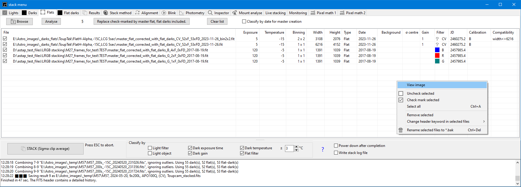
Browse button: use this button to add frames to the list. Frames can also be drag dropped on the form.
Replace check-marked by master flat: This button will combine the individual check-marked frames into a single master flat using the flat-darks loaded in the flat darks tab. So the flat-dark tab should be filled with frames prior to pressing this button. The existing master flats will not be effected. All individual frames will be combined in a master flat with flat-darks included. The flat-dark tab will be cleared after the operation. The user should only combine flat frames and flat-darks with the same gain, temperature and preferable exposure time. If the values are different then this will be recorded in the FITS header behind keyword ISSUES and later reported in the results-tab
Classify during creation
If the list contains frames made with different filters and the option "classify on" flat filter is check-marked then for each filter a different master flat will be created. To automate making a master flat for each observation night you could use the Classify by date for master creation check mark at the top of the tab. This will create master flats for each exposure night from the frame loaded. Flat-darks are not sorted on date because it is assumed they are stable. If you make several flat with different exposure duration (and different filters) you could link them to flat-darks with the same exposure using the option "classify by exposure during master creation.
| Classification-during-master-creation | Filter | Date | Exposure | Gain | Temperature |
| Flat | ✔ | ✔ | ✔ | ||
| Flat-dark |
Classify during stacking
The intention is to keep all master flats here loaded and check-marked. Flat selection on flat filter is automatic by setting the classify on "flat filter" check-mark. For LRGB stacking if a question mark in column "filter" is displayed then filter name in the "Stack method tab" should made the same as in the flat header behind the keyword FILTER. If two master flats only differ in date then the frame with the date closest to the light will be selected. This to ensure that the dust particles pattern matches.
| Classification-during-stacking | Object | Filters equal? | Dates equal? | Exposures equal? | Gains equal? | Temperatures equal? |
| Light | ✔ | ✔ | use nearest | ✔ | ✔ | ✔ |
| Dark | ||||||
| Flat | ✔ | warning (results-tab) | warning (results-tab) | warning (results-tab) | ||
| Flat-dark |
Calibration column
This column will indicate if the flat is calibrated with a dark-flat by the letter B (bias). Use of bias frames are not recommend since modern sensors behaviour can change in the first exposure seconds.
Compatibility column.
This column indicates why the selected flats are not compatible with the light frames. Compatibility issues can be frame width, frame height, sensor gain, sensor temperature, exposure duration. All can be overridden by classify check-mark except for frame width and frame height.
Back to index
Flat darks tab:
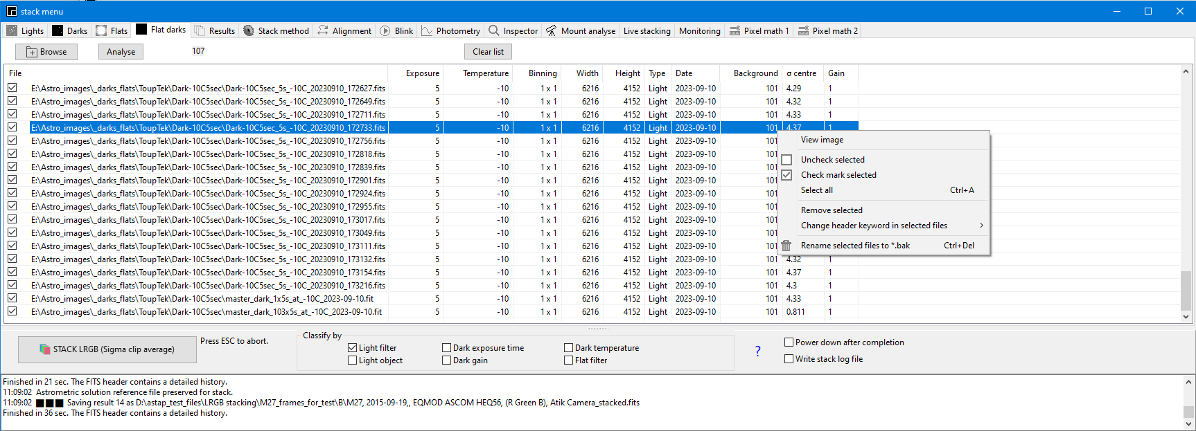
Browse button: use this button to add frames to the list. Frames can also be drag dropped on the form.
After master flat(s) are created the flat-darks tab will be cleared.
Back to index
Results tab.
The stack results are reported
in the results tab. By a double click they can be
viewed the viewer. The number of files and
exposure times are given. With the pop-up menu it is possible
to copy the image file path to the clipboard for use in a file
explorer.
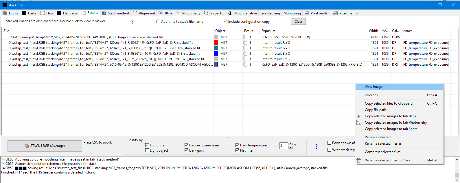
Calibration column
This column will indicate if the stack was calibrated with a dark (D), Flat (F) and flat-dark (B). The S stand for stacked. So ideally it indicates DFBS. Calibration stauts is stored behind keyword CALSTAT.
Issues column
Possible dark frame issues are D_temperature, D_exposure, D_gain. This indicates that the dark sensor temperature, exposure duration and sensor gain are different then the light frame values. Ideally light and dark frames should have been taken with the same sensor temperature, exposure duration and sensor gain settings.
Possible minor flat frame issues are FD_temperature, FD_exposure, FD_gain. This indicates that the flat-dark sensor temperature, exposure duration and sensor gain are different then the light frame values. Ideally flat and flat-dark frames should have been taken with the same sensor temperature, exposure duration and sensor gain settings.
Issues between the darks and lights are more important due to the low light conditions for lights.
These issues are stored in the FITS header behind keyword ISSUES.
Back to indexStack method tab
The best stack option is "Sigma clip average". For only 2 or 3 images or when you are in a hurry or for testing "average"will do.
| Stack method | Stacking | Description | Option σ-factor |
| Average Stacking | ✔ | For fast stacking. Satellite tracks will not be removed. | ✔ |
| Sigma clip average | ✔ | Stacking, satellite tracks will be removed. Reduce the σ factor for more aggressive filtering of the satellite tracks. | |
| Astrometric image stitching mode | Mosaic | This will stitch astrometric tiles. Prior to this stack the images to tiles and check for clean edges. If not use the "Crop each image function". For flat background apply artificial flat in tab pixel math 1 in advance if required. Adapt the mosaic canvas height and width if required, default is 2. | |
| Calibration and alignment of the files only | Darks and flats will be applied. The images will be aligned to the reference image. | ||
| Calibration of the files only | Darks and flats will be applied. | ||
| Average stacking, skip LRGB combine | ✔ | Satellite tracks will not be removed. Stacks based on filter will not be combined to RGB. | |
| Sigma clip average, skip LRGB combine | ✔ | Satellite tracks will be removed. Reduce the σ factor for more aggressive filtering of satellite tracks. Stacks based on filter will not be combined to RGB. |
There are two modes of stacking:
- 1) Stacking of image of a grayscale camera or raw images of a DSLR camera. Stacking in either grayscale of colour goes fully automatic. The program will detect the type of images. Stacking in colour can be forced if the BAYERPAT keyword is not found in the FITS header.
- 2) Stacking of (L)RGB images made with seperate filters. This mode is activated if option Classify by "Light filter" is checked.
Options:
σ factor: This is a factor used by the sigma clip average stacking method to remove outliers like satellite streaks from the stack. For the series lights the standard deviation (σ) is calculated for each pixel and any pixel which is outsider is removed. A typical value of 2 will result in skipping about 4.4% of the pixels. If satellite tracks are not removed you could reduce this factor and more of the satellite streaks will be removed. You could also use the satellite streaks filter. Note that method sigma clip average filtering works better for more images. Try to acquire at least ten images but twenty or thirty images works better.
Auto levels: This is an option to white-balance the final colour result. The stars will be average white and the background sky will be gray.
Normalise OSC flat: This option should normally be switched off. Only if the light source used for making the flats was very reddish or blueish, you could use this option to equalise the red, green and blue levels. Binning is not recommended for flats since individual pixel sensitive differences are compensated by the flat.
Colour smooth: This is an option to smooth the de-mosaic artifacts for all pixels above the noise level. The colours are smoothed while preserving the luminance signal. The same function is available in tab pixel math 1.
Star colour smooth: This is an option to smooth the de-mosaic artifacts of the brighest and medium stars. The colours are smoothed while preserving the luminance signal. The same function is available in tab pixel math 1.
Raw conversion. The program used to convert the RAW file to FITS. It is described here
The program settings will be saved automatically if your either exit the program or start a stack. Settings for Windows are stored at %LocalAppData%\astap\astap.cfg and for Linux at ~/.config/astap/astap.cfg
Stack method tab, stacking grayscale images:
There are no special settings for grayscale images. Classify on "Light images" should be unchecked.
Stack method tab, stacking raw one shot colour images (OSC):
Classify on "Light images" should be unchecked.
RAW images from DSLR cameras /One shot color cameras are monochrome and have to be converted into colour images (after applying darks and flats). This conversion is called demosaic or debayer. First, set the Bayer pattern correctly by loading a raw image (grayscale) in the viewer and try one of the bayer patterns untill the image colours match in viewer. If not, press CNTRL-Z to undo and try a different Bayer pattern.
There are several methods to convert (demosaic/debayer ) the raw image to colour:
- AstroC, colour for saturated stars, similar to the bilinear method but for saturated stars the program tries reconstruct the star colour. Select the range which matches with the value of brightest stars.
- AstroM, white stars, similar to the bilinear method but if there is an inbalance between the 4 red, 4 blue or 2 green pixels it uses luminance only. Effective for unsampled images and stacks of a few images only. Star colour is lost if undersampled but stars will become white.
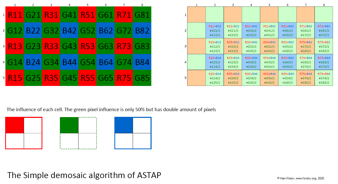
- AstroSimple ©, each R,G, G, B pixel colour information is used in a 2x2 pixel range. Simple but very effective for astro images. Works best for a little oversampled images. Stars have very few artifact if any.
- Bilinear, a basic demosaic method using the colour information from a 3x3 pixel range.
 AstroSimple is © Han
Kleijn,
www.hnsky.org, 2020. and licensed under a Creative
Commons Attribution 4.0 International License.
AstroSimple is © Han
Kleijn,
www.hnsky.org, 2020. and licensed under a Creative
Commons Attribution 4.0 International License.which permits unrestricted use, distribution, and reproduction in any medium, provided the original work is properly cited.
- In general de-mosaiced OSC astro images are suffering from colour artifacts due to the small size of stars and pixel saturation. If the pixels iluminated by a star are saturated, the red, green and blue values will have the same maximum value and the star centre will appear white. In most case this can be avoid by taking short exposures of 60 seconds or shorter.
- Best results are achieved with de-mosaic methods AstroC and Simple.
- In most cases the
option "Auto level and colour smooth" is required for the correct
colour balance and colour smooth. First the three colour channels are
adjusted to make the background colour neutral and the stars average
white. Secondly the bright stars are smoothed. Both actions can be done
manual in the tab pixel
math, option "colour correction" and "smart colur smoothing"
- If the images are under-sampled and the star colour is random after stacking, use AstroM, white stars. Stars will be whiter. Star colour will be lost.
The principle of the AstroSimple demosaic method:
Stack method tab, RAW conversion of OSC images (one shot colour images): To import raw files from a digital camera, ASTAP can either use LibRaw or DCRAW for conversion. You can select it in tab "Stack method". LibRaw has some advantages since the conversion program convert directly to FITS and exposure time, date of exposure and demosaic pattern are written to the FITS header.
The are two option for LibRaw.
- LibRaw (full active area)
- LibRaw (Cropped active area)
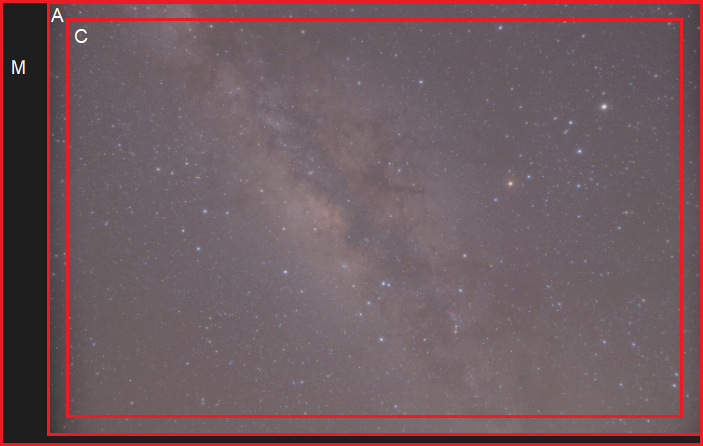
The default value is "LibRaw (full active area). This will extract all active sensor data (e.g. 5202 x3464 pixels) equal A+C below. If you select "LibRaw (Cropped active area)" you get for a little less area (e.g. 5184 x 3456) equals C below.
Note that for stacking all images, light, darks, flats, and flat-darks should be of the same dimensions!
The full area M +A+C (e.g 5360 x 3516) could be extracted using the included command-line utility unprocessed_raw using the -F option but has no purpose in ASTAP.
- A + C: The Active Area, which is the largest area from which a useful image can be formed.
- C: The Crop Area, which is the subset of the Active Area which many raw converters convert into a useful image. The main reason why C is smaller than A is to provide some extra pixels all around for a raw converter's demosaicing algorithm to use.
- M : Masked Area, used by some cameras, especially Canons used a dark.
For stacking of OSC images it is best to start with raw images. The raw colour images look mono, but the program will convert them to colour later in the stacking process. There are four different Bayer patterns. The demosaic pattern can be set in the tab "stack method". Try auto or empirical which will result in the correct colours. A terrestrial image could help find the correct demosaic settings. Load a raw image in the viewer and in tab "Stack method" test conversion with button "Test pattern". Try auto or the four demosaic patterns. If the colours are not correct, just hit undo button or type CTRL-Z to recover and try an other demosaic setting.
Power down option after completion: If stacking takes a long time you could activate this option and the program will be power-down the computer after completion.
Clear , button to remove all files from the list.
|| , button to stop blinking cycle.
⯈ or ⯇ , to start a continuous un-aligned blinking cycle. This is intended to find visually outlier images where guiding has briefly failed.
Back to index
Stack method tab, (L)RGB stacking:
Activating (L)RGB mode:
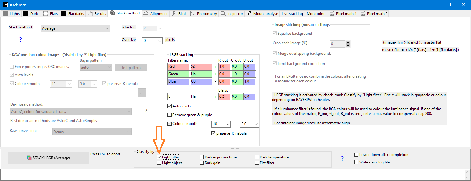
The filter names should match the filter names in the FITS headers. This is the case if in tab Lights the filter column is displaying red, green, blue or gray icon. If there is no match the icon will be a question mark.
Stack method tab, Image stiching method (Mosaic)
Astrometric image stiching is possible with the internal astrometric solver. The reference of each pixel is the astronomical position. So stacking is not done against a reference image but against an position array set by the first image. If if image stitching is selected the SIP option in tab alignment will be activated. This will allow for correction of optical distortions.
.
Here a suggested work method:
- Stack the tiles separately using method "SIGMA-CLIP-average" and use for the alignment the internal STAR alignment method. Inspect the resulting tiles and crop them if required. You can also crop them later automatically with "Mosaic skip outside pixels" Do this for each color separately if you have separate files.
- In tab "stack method" select option "IMAGE STICHING METHOD" and select astrometic alignment using either the internal solver.
- In tab "stack method" check-mark the option "equalise background". If the input images have poor borders, set option crop images larger then 0%.
- Select the files. Most likely the files names
contain "_stacked, so you have the check-mark the files after selection.
- Click on the button Stack check marked images|
- Crop the stacked result using the image crop option in the viewer mouse pop-up menu.
- Adjusted the stretch range and save as JPEG, 90% quality.
Possible error message: Abort!! Too many missing tiles. Field is 11.7x1.3°. Coverage only 14.5%.
This could happens if you have by accident an image from a different series in the collection. The program tries to adapt the canvas to include the outlier but it will be too empthy. Check the positions of the images to stitch and remove any outlier.
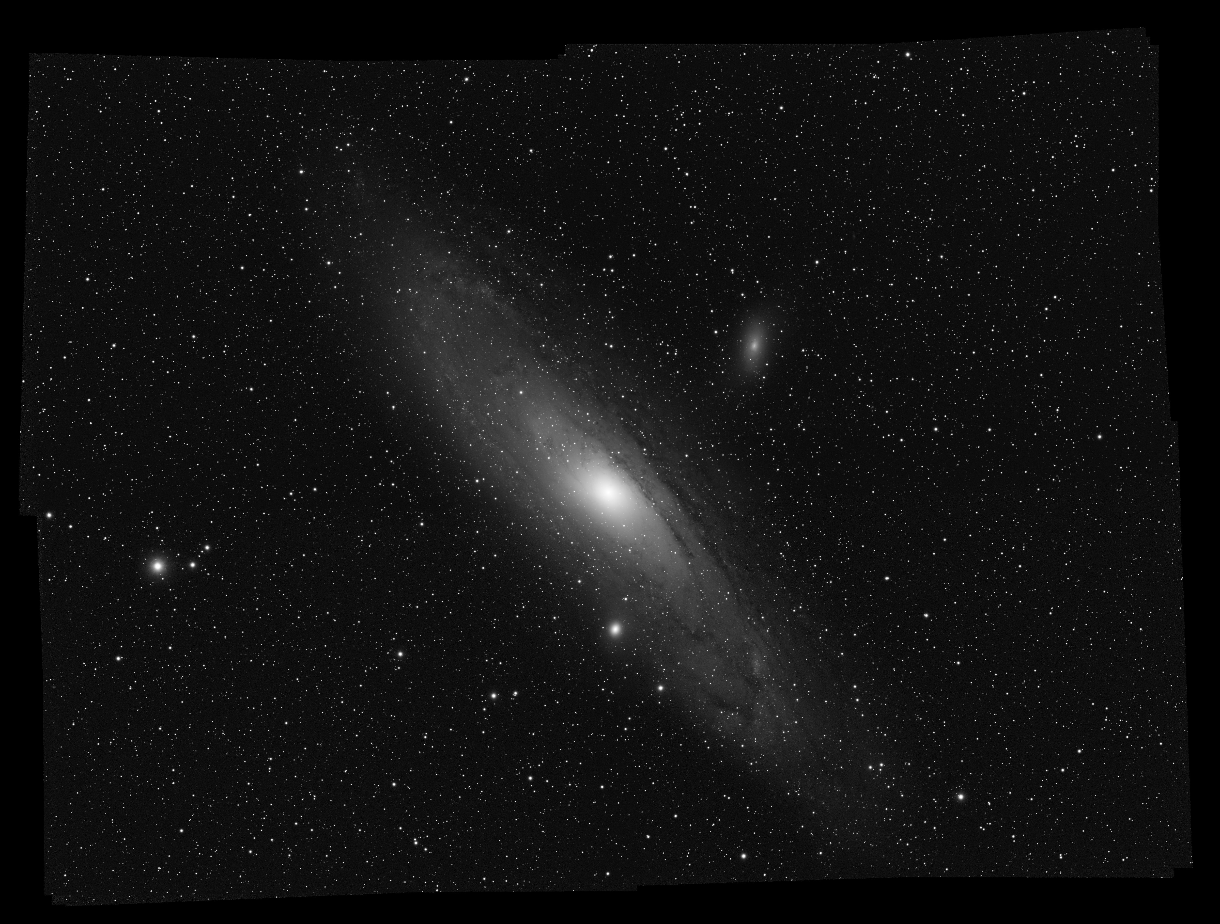
Here an example mosaic x 4 of M31 made with ASTAP:
Here an example of a mosaic build of DSS images:
The size can be reduced by a crop function (right mouse button) later. Making the oversize too large could result in memory overload.
If you have DSLR/OSC sensor and using a monochrome filter like H-alpha, you can split the raw the images in seperate R, G, G, B image using the viewer Tools, Batch processing, Raw colour seperation menu. In case of H-alpha use only the R=red image for future processing.
The alignment menu tab:
For alignment there are four options, internal star alignment, native astrometric solver, manual alignment or ephemeris alignment. For mosaic building you have to use the internal astrometric solver.
Internal star alignment
This internal star matching alignment is the best and fastest option to stack images. It is not suitable for mosaics. No settings required; fully automatics alignment for shift in x, y, flipped or any rotation using the stars in the image. It will work for images of different sizes/camera's with some limitations.
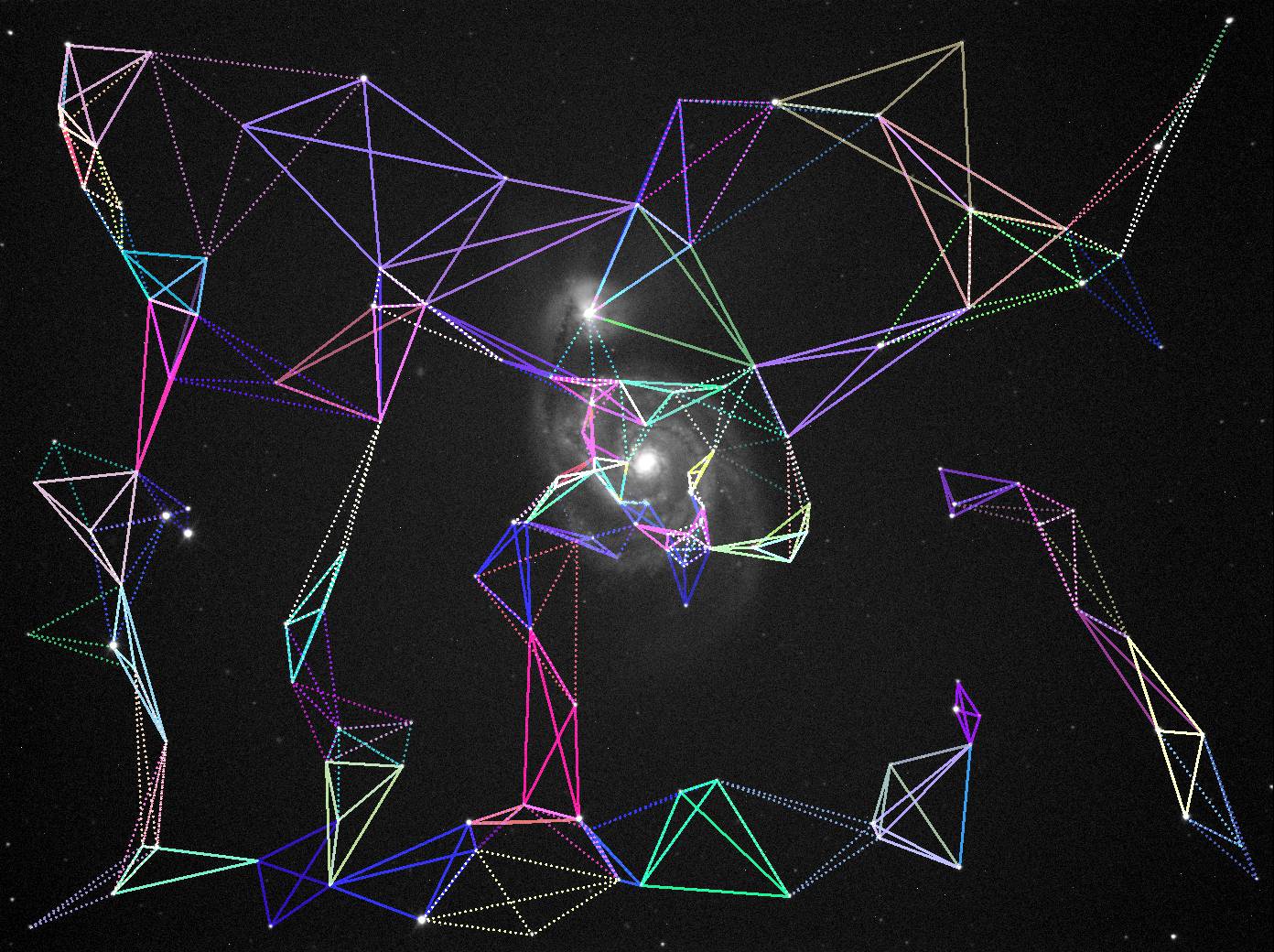
The program combines four close star detections into an irregular 2D tetrahedron or kite like figure (and compares the six irregular tetrahedron dimensions with irregular tetrahedrons of the first/reference image. It selects at least the three best matches and uses the centre position of the irregular tetrahedrons in a least square fitting routine for alignment. The four star detections are called a quad. The six geometric distances are used to construct a hash code.
There are only three relevant settings, but normally you don't have to change them.
- Hash code tolerance Quads matching tolerance. Default setting 0.007. Leave this at 0.007 or 0.005 unless you have severe optical distortion. If you have too many false detections then set this lower.
- Maximum number of stars. Number of star detections used to build quads. Default setting 500. In some cases like for images with a lot of hot pixels you could set it lower to avoid false detections.
- Ignore
stars less then [HFD].
Setting for stack alignment to filter out hot pixels out of the star
detection. Default value 0.8. Single hot pixels have a HFD of
less then 0.8. { 2*(0.5/PI())^0.5=0.798 }
The following image shows the selected quads. The six geometric distances between the four star detections form an irregular tetrahedron and will be used as a hash code:
The matching process is described here Background info, how does the ASTAP astrometric solving works internally
Alignment tab, astrometric alignment.
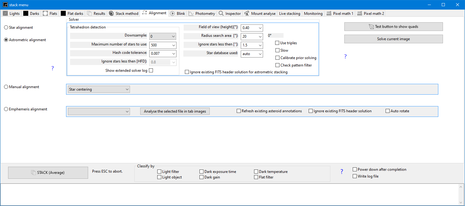
Internal astrometric solver (plate solver). This works with the same four star quad detection as for the Star alignment option. The found quads are compared with the star database (to be installed in the program directory). In most cases the star alignment is prefered above the astrometric alignment.
It has the following settings both applicable for the astrometric solving and astrometric alignment:
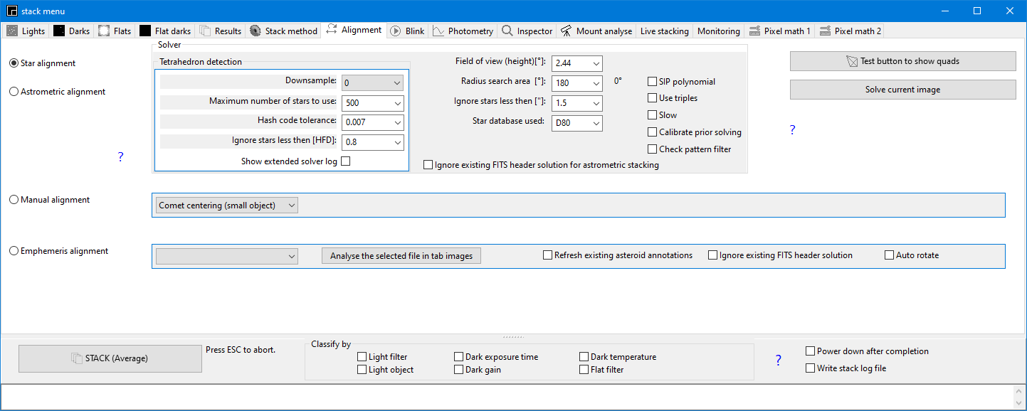
Tab astrometric alignment and solver settings:
- Field height: This is the square size of the star field in degrees used for detection and will be set automatically for most FITS files. It should equal to the image height in degrees. If unknown, you could try initaly the option "auto".
- Radius search: Search radius in degrees. If there is no match, the program will move the search field around in a square spiral and increasing the distance form the initial position up to the radius specified. A radius of 30 degrees could be searched in a minute.
- Ignore star less then ["] Any star with a HFD below this value will be ignored. This will filter out hot pixels. Default setting 1.5".
- Star
database used: If you select "Auto" the
following logic will be used:
FOV>20° ==> if exist W08
ELSE
FOV>6° ==> if exist G05
ELSE
FOV<0.5° ==> if exist D80
ELSE
==> if exist V50, D50, D20, D05, D80, G05 - Downsample: For large images, the downsampling will speed up the solving and increase the signal noise ration of the stars. Default position is 0 equals auto. Any image with a height dimension above 2500 pixels will be binned 2x2. Also colours are combined to monochromatic so this option is beneficial for colour images. Avoid too much binning. Resulting height should be 960 pixels or higher. In mode downsampling auto=0 any pixel scale less then 1"/pixel is binned to get a larger pixel scale. This is beneficial for the typical astro images but for images taken by a telescope high on mountain with superb seeing you might choose a fixed downsample factor.
- Maximum number of stars to use: Number of star detections used to build quads. Default setting 500. If the database density is not sufficient the maximum number of stars will be reduced automatically.
- Hash code tolerance: Quads matching tolerance. Default setting 0.007. Leave this at 0.007 or 0.005 unless you have severe optical distortion. If you have too many false detections then set this lower.
- SIP coefficients: Using this option the solver will add 3th order SIP polynomial coefficients to the header to cope with image distortion. This option is not relevant for stacking since the distortion for each frame will be the same. It is only important for positional astrometry.
- Use
triples. Experimental option for images with a low star
count only. Default unchecked.
- Slow. This will force a 50% overlap between search fields. Default unchecked. Use this in rare cases where solving fails while still many star are detected. If applied this will slow down blind solving.
- Solar drift compensation This is a special option to stack aligned on minor planets or faint moons. The stack process will align on the stars but with a angular movement correction you have to enter theα and δ rate in arcseconds/hour. Using the date of observation, the solar object will be sharp in the stack while the stars will form streaks. This allows imaging faint objects especially faint moons where no ephemerides are available. For common solar objects you better use the option ephemeris alignment. Angular movement rate can be extracted from JPL Horizons using the custom output option "Rates; RA & DEC". The rates from JPL Horizons have to be entered without any modification.
The internal plate solver works best with raw unstretched and sharp images of sufficient resolution where stars can be very faint. Exposures should 5 to 300 seconds. Heavily stretched or Photoshopped images are problematic.
For those who are interested: Background info, how does the ASTAP astrometric solving work internally
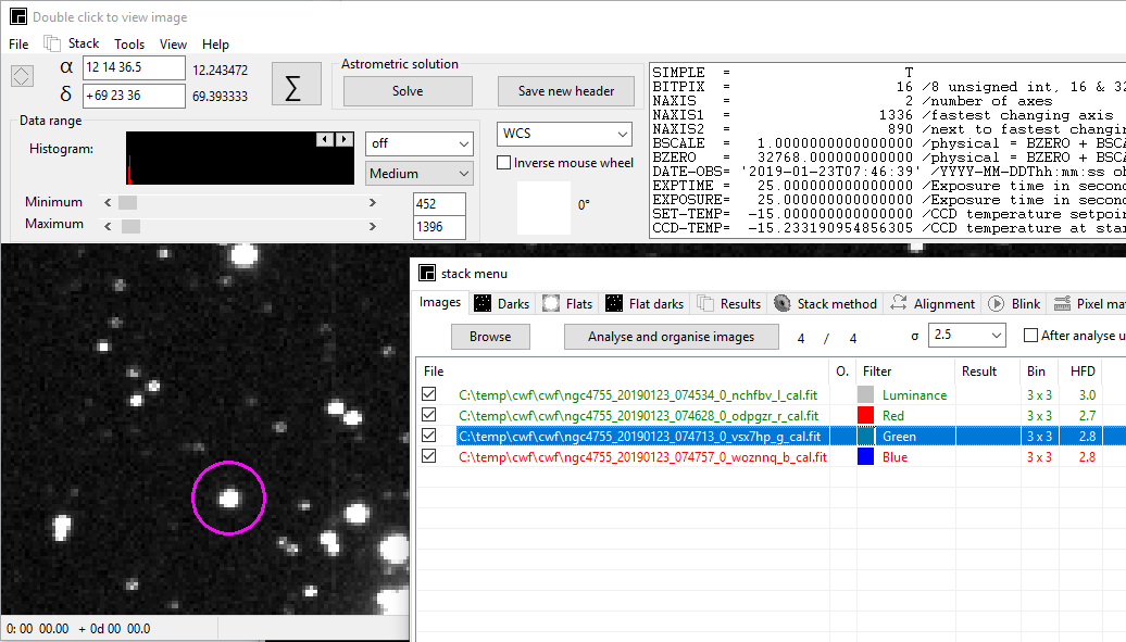
Alignment tab, manual alignment.
Manual alignment
This option allows alignment of the images based on a single star, asteroid or comet. If this option is activated, the list of images in the image tab turns red. Double click on each image in the list and click on the star/comet or asteroid to be used as reference. This object is then marked with a little purple circle. The position will be auto centered. (and the X,Y position will be added to the list) A poor lock is indicated by a square. If so try again until it is a circle. If all images in the list are turned green, so contain a x,y value, then click on the Stack button.
Options:
- Star centering
- Comet centering
- No alignment
For objects which are moving in the sky, select the stack option "average" and not the "sigma clip" option.
For manual alignment there is an option in the pop-up menu of tab light to select the next alignment stars automatically:
- Select an alignment star in the first image.
- Select all images in the Lights tab.
- Select from the pop-up menu of the Lights tab "Auto alignment star for selected images"
- If it stops halfway, then it doesn't lock on that image star halfway. Select manually in that image the same star and try again or continue with the next images.
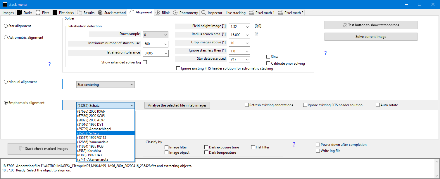
Alignment tab, ephemeris alignment
Rather then manual selecting the reference point it is also possible to use the ephemeris of an asteroid or comet. To align by ephemerides go through the follow steps:
Preparation:
- Configure and test the viewer Asteroid & Comet annotation menu shortcut CTRL+R
- Select ephemeris alignment
- Browse for all the images in the image tab and add if available the dark, flats.
- Press the button Analyse the selected file in the tab images.
- Select from the combo box the asteroid or comet to align on. See screenshot below. If no objects are listed then check if there is a comet and/or an asteroid database available. See the Asteroid & Comet annotation menu, shortcut CTRL+R') If still none, then increase the limiting count and/or limiting magnitude in the same menu.
- Hit the Stack button.
- After the stacking is finished it is possible to annotate the result.
Only the solar object selected will be sharp. The stars will form trails. There is an experimental stack method to have both sharp but it will use only the stars of one image.
This tab allows you to blink images to show movement and to export to video.
With the blink pop-up menu it is also possible to "track and stack" selected images aligned on a specific solar object for a better signal to noise ratio. The object velocity (i.e., movement~~) is neutralised by the stacking algorithm. In the final image, positions and accurate date and time of these objects can be retrieved from the stacked image using the viewer pop-up menu "Mpc1992 report line".
Button functionality:
Blink comparator. This option allows rapidly cycling (blinking) through the images taken of the same area of the sky at different times. This will allow the user to more easily spot moving objects. While blinking the result can be demosaiced (slow) if the "auto demosaic" option in the viewer is activated.
|| , button stops the blink cycle.
⯈| , button starts one blink cycle.
⯈ , starts a continuous blink cycle.
⯇ , continuous blinking backwards.
☑ Align images. With this option checked, the images will be aligned using star alignment. The alignment will be refreshed after pressing "clear alignment"
☑ Time stamp. With this option checked, a time stamp from the header will be written to the bottom of the image. If the displayed image is saved as FITS, this time stamp will be written to the saved image.
Clear, button to remove all files from the list.
Export
video
This button will export the blink result to an uncompressed
.y4m
video file (YUV4MPEG2). For OSC images, activate the
viewer the "auto demosaic" option. The menu will ask for a
video
file name and
desired frame rate per seconds. Contrast will be as set in the viewer.
Compression can be achieved in
an external program like VLC or left to YouTube. If
time-stamp is checked then the time stamp will be written to
the video.
Export
aligned This button allows the creation of
aligned FITS images. If blinking with alignment
works well, stop blinking and hit this button All images will
be copied aligned to new files ending with
"_aligned.fit". Alignment will be done against the first image
in the list after
alphabetic sorting. If time-stamp is checked then the time
stamp will be written to the aligned images.
To select a different reference image for alignment do the following, Analyse , Clear alignment , click on the image to be reference to give it a blue marking, then click on ⯈
(Re)annotate (&solve) , This re-annotate the images with e.g. the minor planets and comets. Use this if the annotation is wrong due to an outdated MPC file.
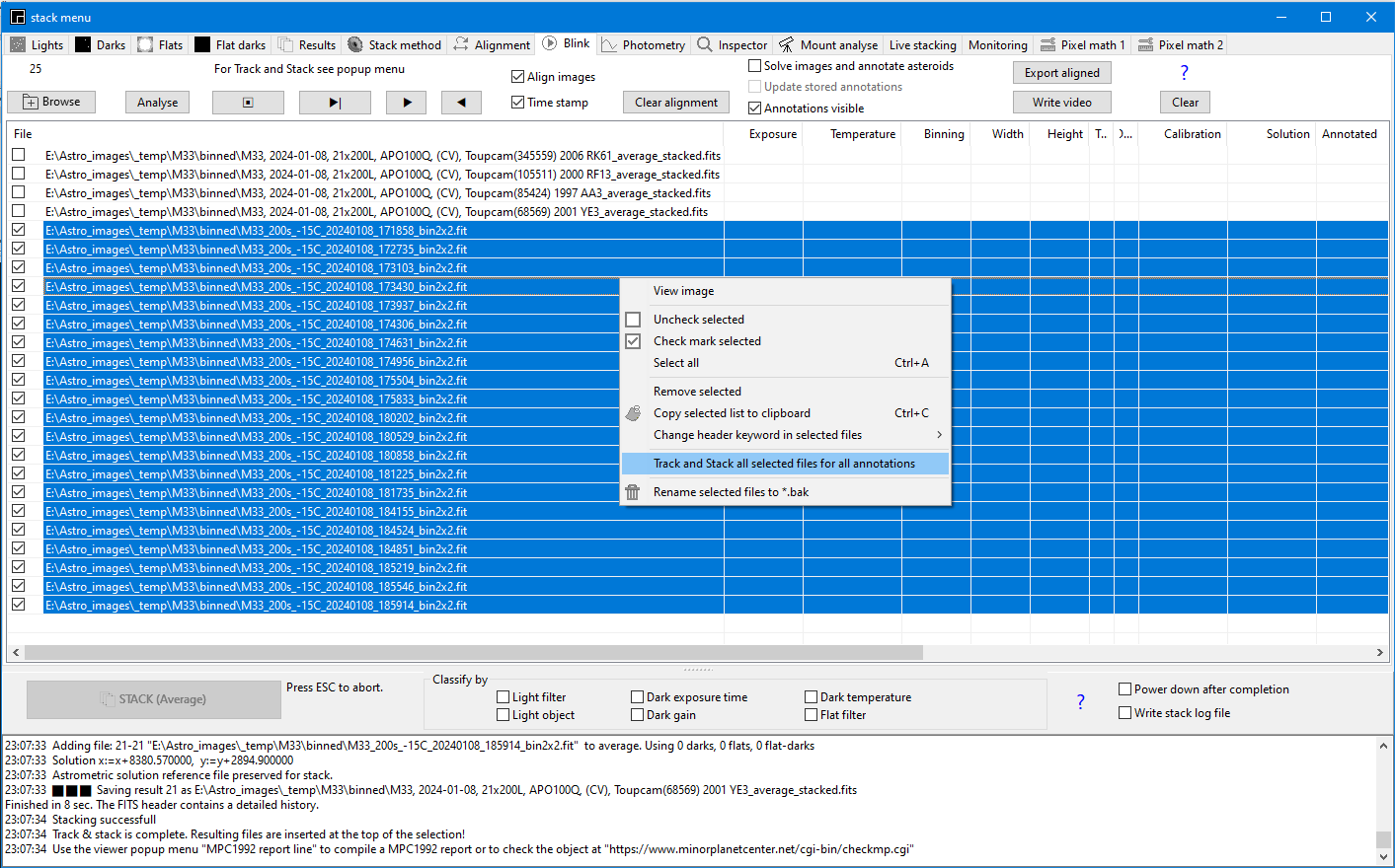
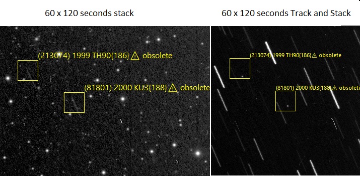
This pop-up menu of the blink tab allows you to track and stack all annotated minor planets and comets in separate stack images of 299x299 pixels for easy identification. The Track and Stack will improve the signal to noise ratio since all flux will be concentrated at one spot. The minor planet will be stacked to a single position and the stars will form streaks. This goes fully automatically based on the MPC database. The number of minor planet annotations is set in the viewer menu "Asteroid and Comet Annotation" shortcut Ctrl+R.
Track and Stack will work for OSC/DSLR images (v2024.03.08) It will produce stacks in colour. If you apply the bin 2x2 button prior to track and stack then the result will be a mono stack. This mono stack could be a little more astrometrically correct.
"Track and Stack" demonstration on Youtube
Usage:
- Load the images in the Blink tab.
- Display one image and check the asteroid and comet annotation (Ctrl+R). Set in this menu the limiting number of minor planets and/or limiting magnitudes correctly to show only minor planets within reach of your telescope and camera. If your MPCORB database is too new (+100 days) or too old (-100 days) all the annotations will end with the remark "⚠obsolete".
- Select the group of images you want to track-and-stack and release the right mouse button to get the pop-up menu and select "Track and Stack all selected files for all annotations. Assume 10 minor planets are annotated due to the setting in the viewer asteroid and comet annotation menu (shortcut Ctrl+R) Then all images will be solved, annotated and stacked in ten separate images. For each minor planet one dedicated tracked stack will be created using the calculated velocity of that minor planet. So the minor planet will be star-like shape independent of the movement and the stars will form streaks. The new stacks will be added in the list before the selected files. Faint minor planets will stay invisible, but some will get enough signal to noise ratio to be visible in the stacked image.
- Double click on one of the ten stacks, move the mouse pointer to the minor planet of interest and select the viewer pop-up menu, "MPC1992 report line".
- Optionally, you could paste the report line into the MPC checker page for confirmation.
This photometry tab allows aperture photometry of variable stars.
1) Load the images in the photometry tab using the Browse button. If you have a SeeStar telescope use these SeeStar guideline.
2) Optionally you could use Analyse button or + button to analyse or analyse+ the images.
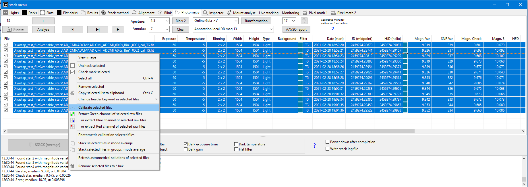
3) In case calibration is
required and/or splitting raw OSC images in green /blue see the photometry popup menu.
This allows calibration and raw splitting of the images from the photomotry tab.
4) Select either:
a) Manual star selection. The classic method. After selecting this option, click on one of the images in the list and select up to 10 stars to measure. Identification which are variables, check or comparison star(s) will be done later in the report.
b) Measure all annotated SNR>30 (All stars existing in the AAVSO VSX and VSP database are measured down to the SNR set.
c) Measure all stars SNR>30
5) Press the ⯈| (play)button to measure all images. The program will do the following:
Cycle 1: Find an astrometric solution for all selected images and write the solution to the FITS file header.
Cycle 2: In a second cycle, the program will identify stars in the image and measure the star flux against the V50 local or online star database. The columns on the right side are filled with the measured magnitudes against the star database. These first values will be pretty accurate but are in principle still instrumental magnitude value and not calibrated against selected comparison stars. If the online database is selected, the reported instrumental magnitudes will be calibrated against the transformed Gaia magnitudes indicated by a corresponding icon else against the local V50 star database (to be selected). For the final result is doesn't matter since these initial instrumental magnitudes are later corrected with the comparison stars.
6) Optionally, if you have imaged and loaded standard field images, press the Transformation button to find and save the transformation coefficients for your system for later use.
7) Press AAVSO report to open the report window. In the report window select one or more variables, one or more comparison stars and a check star/
8) If it all looks correct, click on create the report. If you see an outlier, you can use the graphic popup menu to select the corresponding image to inspect.
For stars suffering from nebulosity like R Mon (NGC2261) use the special option "Disable star autocenter". This option is not stored.
Youtube videos:
- Photometry with SeeStar telescope using ASTAP for processing .
- Photometric transformation using the ASTAP program.
| Viewer | Photometry tab and report | |||||
| Filter used for imaging | Reference star database | Reported magnitude viewer status bar | Reported magnitude listview | Reported magnitude with option Gaia ensemble | Reported magnitude using COMP star(s) | Transformation correction (only required for poor filters) |
| CV | D80 | BP (Gaia blue) | BP (Gaia blue) | BP (Gaia blue) | BP (Gaia blue) | - |
| B | D80 | Erroneous BP | Erroneous BP | Erroneous BP | Erroneous BP | - |
| V | D80 | Erroneous BP | Erroneous BP | Erroneous BP | Erroneous BP | - |
| R | D80 | Erroneous BP | Erroneous BP | Erroneous BP | Erroneous BP | - |
| CV | V50 (contains only V) | Erroneous V | Erroneous V | Erroneous V | - | - |
| TB (OSC split) | V50 | Erroneous V | Erroneous V | Erroneous V | TB poor | B |
| TG (OSC split) | V50 | Erroneous V | Erroneous V | Erroneous V | TG | V |
| TR (OSC split) | V50 | Erroneous V | Erroneous V | Erroneous V | TR poor | R |
| B | V50 | Erroneous V | Erroneous V | Erroneous V | B accurate | B accurate |
| V | V50 | V | V | V | V accurate | V accurate |
| Rc | V50 | Erroneous V | Erroneous V | Erroneous V | R accurate | R accurate |
| SI | V50 | Erroneous V | Erroneous V | Erroneous V | SG accurate | SG accurate |
| SR | V50 | Erroneous V | Erroneous V | Erroneous V | SR accurate | SR accurate |
| SG | V50 | Erroneous V | Erroneous V | Erroneous V | SI accurate | SI accurate |
| CV | Gaia online | BP (Gaia blue) | BP (Gaia blue) | BP (Gaia blue) | - | - |
| TB (OSC split) | Gaia online | TB poor | TB poor | TB poor | TB poor | B |
| TG (OSC split) | Gaia online | TG | TG | TG | TG | V |
| TR (OSC split) | Gaia online | TR poor | TR poor | TR poor | TR poor | R |
| B | Gaia online | B | B | B | B accurate | B accurate |
| V | Gaia online | V | V | V | V accurate | V accurate |
| Rc | Gaia online | R | R | R | R accurate | R accurate |
| SI | Gaia online | SG | SG | SG | SG accurate | SG accurate |
| SR | Gaia online | SR | SR | SR | SR accurate | SR accurate |
| SG | Gaia online | SI | SI | SI | SI accurate | SI accurate |
Photometry topics:
Press AAVSO report button to open the report window
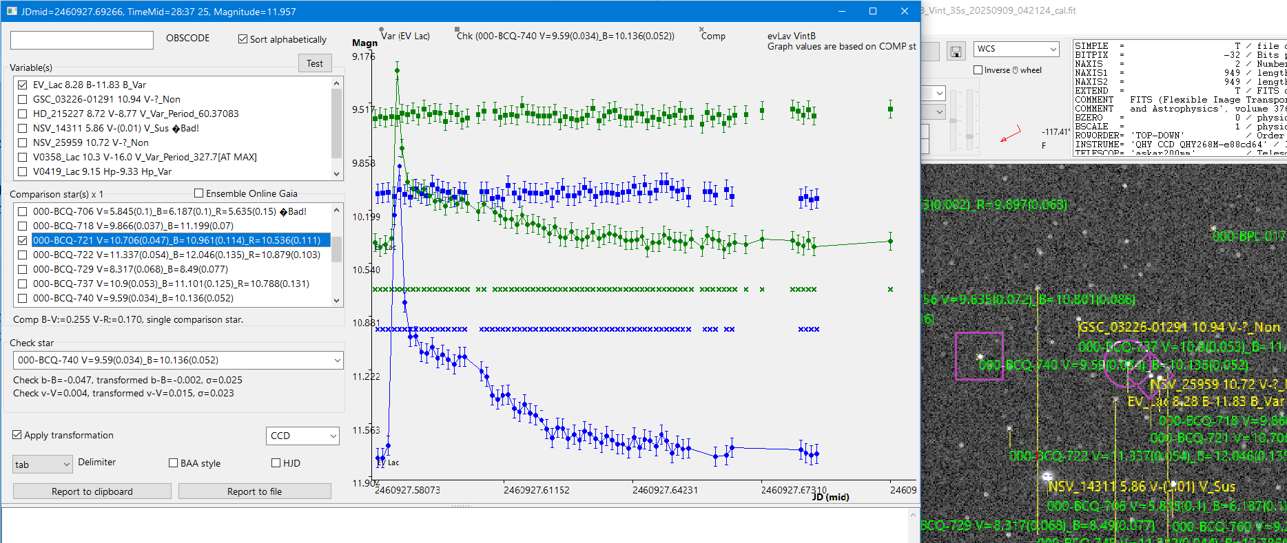
In the report window select one or more variables, one of more comparison stars and a check star. Only the check stars are used for the report. The star selection is reported back into the viewer with purple annotations.
Enter your four digit observer code in the top entry.
After selecting the variable(s), comparison star(s) or check star the trend graph is updated. The uncertainty of the check star is used for the uncertainty bars for both the variable and check star. If one of the measurements is an outlier, you could find the corresponding image with the popup menu of the graph and inspect it. The graph trend colours are similar as the filter colours. The graph can be copied to the clipboard using the same popup menu.
Check the transformation check-mark if you have measurements in two colours, B & V or V & R and established your transformation coefficients with images of a standard field.
As a quality check the b-B and v_V difference of the check star are reported below the check star selection. Small letter b or v stand for measured values. Capital B or V stands for documentend magnitudes. In the the quality check report lines also the check star magnitudes are transformed indicating if the transformation is working correctly. The check star values in the report are not transformed according the report guidelines.
Check the check star error(s)
so the b-B or v-V values of the check star are reported below the check
star selection. Instead of
the comparison star(s) you could select the star Gaia database
as comparison (reference) but this be in general
less accurate. Click on either on
"Report to clipboard" or "File".
If the stars are selected and the graph looks correct, you can create the report with either "Report to clipboard" or "Report to file". The report text and graph are saved to the same directory as the image files. The report format is either according to the AAVSO Extended file format or BAA style as selected.
Automatic photometry. Measure all
stars with annotations
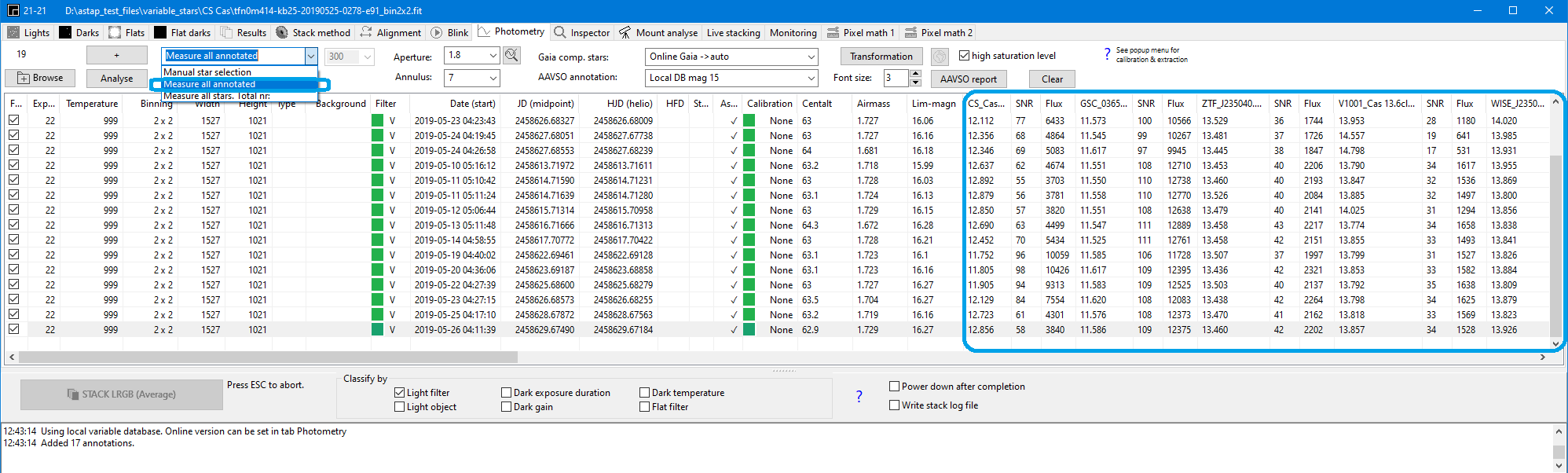
Once measured any of the measured Var and Check stars can be selected in the combo boxes of the AAVSO report window.Alternatively you could copy all data to a spreadsheet by Ctrl-A (select all rows) and Ctrl+C (copy ) and paste it into a spreadsheet for further processing.
The photometry pop-up menu:
Pop-up menu of photometry tab:
Change header keywords of selected files: The pop-up menu has an option to update a keyword in multiple files if required. Select the files to modify and select the pop-up menu with the right mouse button. If you type for the new keyword value in capital letters DELETE, then the keyword will be removed from all file headers.
If the keyword DATE-OBS is typed then the program will request a time shift in hours or a fraction of an hour. This could be used to correct a recorded time of observation. The old DATE-OBS value is stored behind a new keyword like TT120619 for recovery by renaming it back to DATE-OBS. See this screenshot astap_keyword_menu.png
Extract green pixels. Select all files in the Photometry tab and from the pop-up menu select "Extract green channel". Images will be converted to new images with filename ending "_cal_TG.fit". The RGB pattern should be correct. Check prior in the stack method tab with the "test pattern" button if the default de-Bayer pattern "auto" results in the correct result. This works best with terrestrial images otherwise select a manual de-Bayer pattern.
Refresh astrometric solutions of selected files. If the images are not solved yet, press the "Refresh astrometric solutions" button This is required to identify the stars for photometric calibration against the V50 star database. If no solutions are found, check the image "Field of view (height)" in degrees in the "alignment" tab and check the initial α,δ position in the viewer. If solving fails, go through the check list for solving.
Stack ALL files in groups, mode average. This option will stack the files in groups of 2, 3, 8, .. as you specify. This will improve the signal-to-noise ratio of the imaged stars but reduce the number of observations. This routine will process all checked files in the photometry tab. Prior to stacking the files will be automatically sorted on filter and secondary on JD-mid (date). The original files are unaffected but are removed from the list.
Back to photometry_index
Here is an example of an exoplanet transit measured using the photometry tab:
![]()
A demonstration is available on YouTube: Measure variable stars
With ASTAP you can transform your data to the standard system Johnson-B, Johnson-V and Bessel-R. For transformation the minimum input is two colour channels.
Monochrome camera with Johnson-B, Johnson-V and Bessel-R. Ideally the input comes from a system with Johnson-B, Johnson-V and Bessel-R filters to eliminate the last differences. They will be transferred to come closer to Johnson-B, Johnson-V and Bessel-R magnitudes.
DSLR/OSC cameras: Alternatively the input channels could come from a raw image from a DSLR/OSC camera. These raw images can be split into raw red, green and blue color channels called TR, TG, TB. The TG filter magnitudes transform well to V. However TB and TR filter magnitudes do not transform as well for targets of very blue or red colors, Therefore, your transformed B or R magnitudes may not be as accurate as desired. It may be more reliable not to transform TB or TR magnitudes although this is a conclusion of much continuing debate.
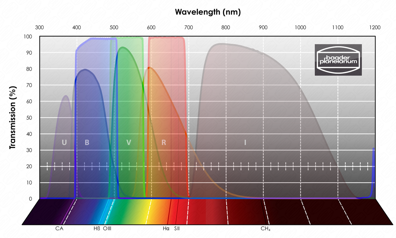
Monochrome cameras with RGB filters: Below are the transmission curves of Johnson-B, Johnson-V and Bessel-R filters of a well know supplier compared with the more square pass band RGB interference filters. Overlapping passbands (like Johnson/Bessel UBVRI) are advantageous for broadband photometry where accurate colors and spectral energy distributions are key but RGB can still be used.
| Name | RA | Dec | Mag_Range | Diameter_(arc min) |
| NGC 1252 | 03:10:49 | -57:46:00 | 8 – 15 | 300+ |
| M67 | 08:51:18 | +11:48:00 | 7 – 16 | 74 |
| NGC 3532 | 11:05:39 | -58:45:12 | 8 – 13.5 | 30 |
| Coma_Star_Cluster/Melotte_111 | 12:22:30 | +25:51:00 | 5 - 10 | 450 |
| M11 | 18:51:05 | -06:16:12 | 8.5 - 17 | 20 |
| NGC 7790 | 23:58:23 | +61:12:25 | 10 - 20 | 7 |
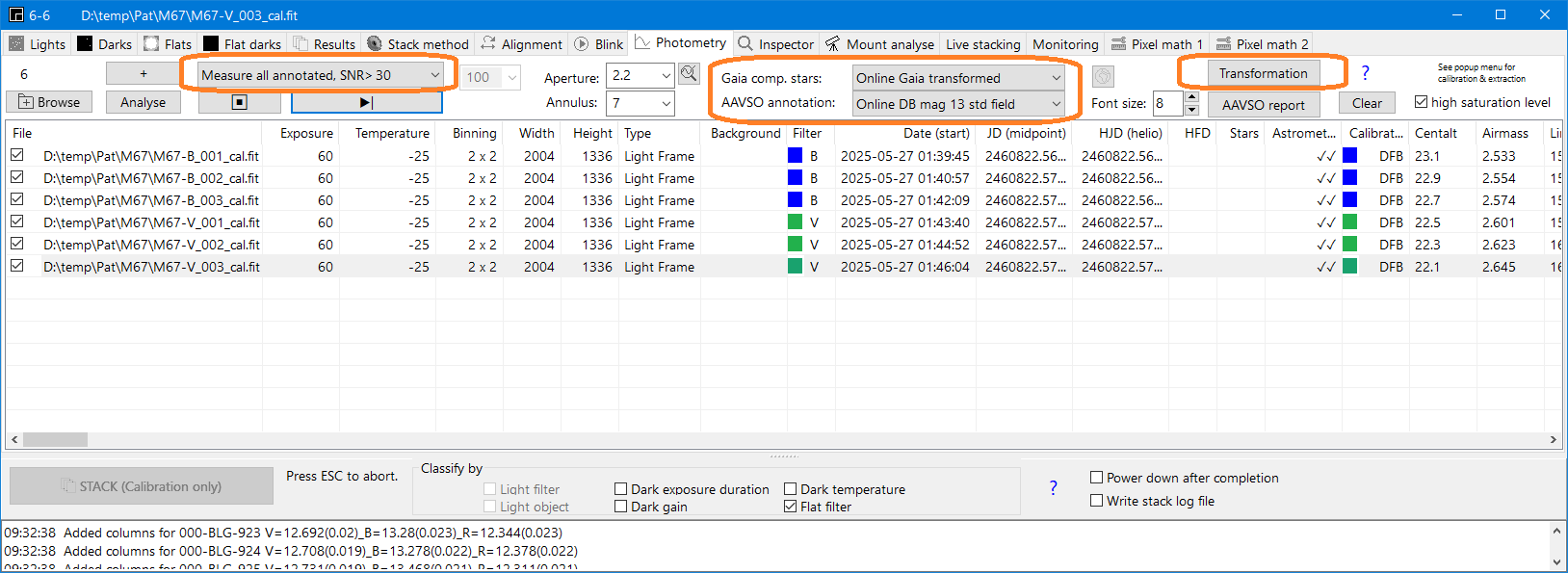
The whole procedure to establish the transformation coefficients is as follows
- Get images of a standard field made with B, V filters or DSLR camera.
- Load them in the ASTAP Photometry tab.
- Select in tab photometry for AAVSO annotation either the local database or the online standard field like "Online DB mag 13 std field".
- Select in the Photometry tab for the Gaia comp stars "Online Gaia". This is required for the blue and red filter images. The local database contains only the Johnson-V magnitude.
- In case of a DSLR images use the photometry tab popup menu to split them in TR (red), TG (green) and TB (blue) For DSLR cameras it is important to keep the stars a little out of focus since red and blue sensitive pixels are only one-quarter of the pixels.
- Calibrate the images with dark and flat & flat-dark if possible.
- Press the transformation button. If required the image will be solved. Check the found coefficients.
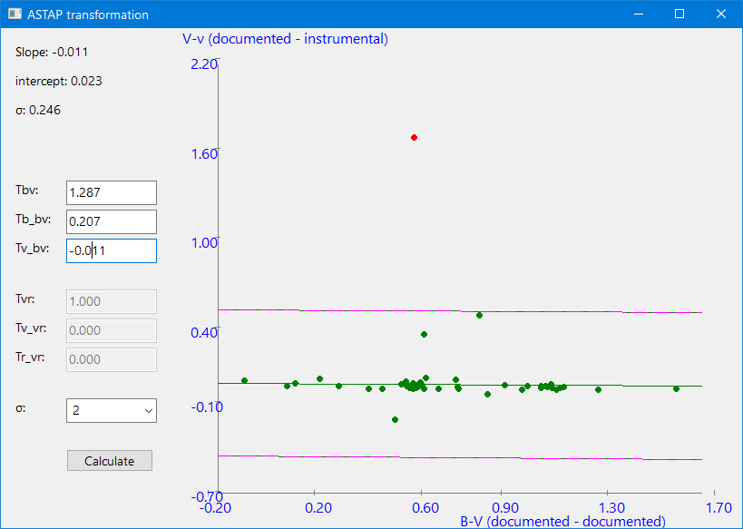
In case the images are taken in two colours (B, V in this case) the transformation window will show three transfer functions:
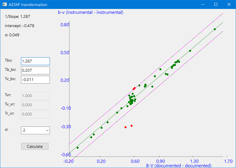
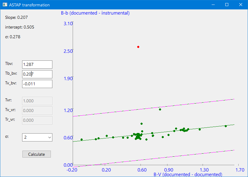
b is the instrumental blue magnitude measured of the stars..
B is the documented blue magnitude of the stars..
v is the instrumental v magnitude of the stars.
V is the documented v magnitude of the stars.
With the σ setting in the transformation menu it is possible to adjust the outlier removal. The stars are marked with a green dot which changes to a red dot if ignored as an outlier. The green line is the interpolation line of the measurements.
The colour of the star is defined by B-V. If the B and V magnitudes are the same then B-V is zero and the star that would appear white to the human eye. This corresponds to a surface temperature of about 10,000 K, which is characteristic of an A0-type star. Vega, one of the brightest stars in the night sky, has a B–V of about 0.00.
The slope of the transfer function B-b and V-v as a function of the documented star colour index B-V is what we want to compensate through transformation. So if a star is blueish (B-V<0) or reddish (B-V>0) then the measured magnitudes could have a measuring error depending on the slope of the curve.
The above graphs show an almost perfect V filter with a slope of only -0.011. The blue filter has a slope of +0.207. The measurement accuracy will increase if transformation is applied for the magnitude measurements in blue.
The correction to be applied to the measured V magnitudes is Tv_bv⋅(B-V) The problem is that the B-V (the documented colour index) of the target (tgt, the variable) is often not known.
But the instrumental magnitude difference b-v can be measured. Then the full transformation correction becomes Tv_bv⋅[(b−v)var−(b−v)comp]⋅Tbv
Without transformation
Δv is the instrumental magnitude of the variable minus the instrumental magnitude of the comparison star or vvar- vcomp
Vcomp is the published V–magnitude of the comparison star
With transformation
Δ(B-V) is the difference in the standard color of the variable versus the standard color of the comparison star and is equal to Tbv * Δ(b-v). In other words, you can derive Δ(B-V) by multiplying your color transform by the measured color
difference between the variable and comparison star, Δ(b-v). Then formula 2) can be written as:
- : how different the instrumental colors of the variable and comparison star are
- : converts instrumental color difference → standard color difference
- : tells how much a difference in shifts the V magnitude in the system
Pairing: For a V image, find a B image with the nearest time stamp.
Instrumental Δv := -2.5 * log10(Flux_v_var/∑Flux_vcomp)
Instrumental (b−v)var := -2.5 * log10(Flux_bvar / Flux_vvar)
Instrumental (b-v)comp := -2.5 * log10(∑Flux_bcomp / ∑Flux_vcomp)
Catalog Vcomp:= -2.5 * log10(∑(10^-0.4Vcatalogcomp))
You can combine Δv+ Vcomp in (4) and write it as:
Vvar=Δv + Tv_bv * Tbv *((b-v)var - (b-v)comp) +Vcomp (4)
equals
Vvar= -2.5 * log10( Flux_vvar*∑(10^-0.4Vcatalogcomp)/∑Flux_vcomp) +(Tv_bv⋅Tbv⋅[(b−v)var−(b−v)comp]) (5)
Where
Flux_vvar is the measured flux of the variable star.
Flux_vcomp are the measured flux values of the comparison stars.
Vcatalog_comp are the catalog magnitudes of the comparison stars.
The found transformation coefficients will be stored in the ASTAP configuration file astap.cfg for later use. These coefficients do not need an update for at least a few months or much longer.
If you want to report in V transformed you will need only one measurement of the Var in B. So your image filter sequence could be:
B, V, V, V, V, V, V, V, V, V, V, V, V, V
or
V, V, V, V, V, V, V, V, V, V, V, V, V, B
or
TB, TG, TG, TG, TG, TG, TG, TG, TG, TG, TG, (TG are the green sensitive pixels of an OSC/DSLR image)
All above will result in a transformed V series even the TG series. It is important that at least one V image has a similar time stamp as the B image since this pair will be used for the (b-v)var measurement.
To report both in B & V you will need the following image filter sequence:
B, V, B, V , B, V, B, V, B, V, B, V, B, V, B, V
ASTAP will search for an image pair B & V with the closest Julian Day since the variable magnitude could change over time..
The actual transformation process
The usage is as follows.
- Load into the photometry tab images made with B, V (or R) filter.
- Select in the photometry tab for the AAVSO annotation online or local. The local DB is only suitable for B & V or TB & TB measurement. For R or TR use the online version.
- Select in the photometry tab for the Gaia comp "Online Gaia " or local V50. The database selection is not essential unless you choose later Gaia ensemble as comparison.
- In case of a DSLR images use the photometry tab popup menu to split them into TR (red), TG (Green) and TB (blue) For DSLR it is important to keep the stars a little out of focus since red and blue are only captured by a 1/4 of the pixels..
- Select "measure all in the photometry tab"
- Press the play button. The imaged stars are now
measured. The
listview will now contains the instrumental magnitudes based
on the star
database. The values are reasonably correct using the star database for
a first correction.
- Press AAVSO report.
- Uncheck "Gaia ensemble". This
will allow in the final report a final correction of the
instrumental magnitudes using the
selected comparison stars.
- Check "transformation"
- Select variable, comp stars and check star.
- Press either "Report to file" or "Report to clipboard".
Below is an example of a report. The blue coloured text indicates the change after transformation. The original filter is mentioned in the comments since after transformation DSLR bands TB, TG, TR will be change in B, V, R in the output..
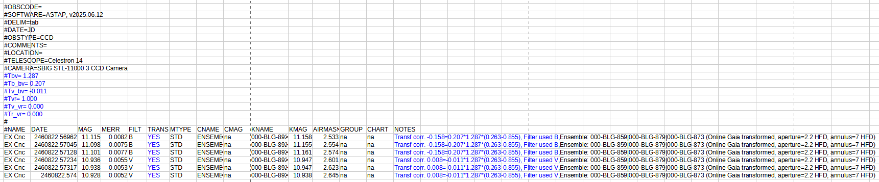
Back to photometry_index
Back to index
Test your transformation
It is important to test your setup. In the AAVSO report window there is a button "Test mode" . Use this to test the transformation process and achieved accuracies.
In the report windows the difference between the measured and documented magnitude of the check star are reported. Also the error after transformation of the check star. This transformed check star magnitudes are not reported in the report and only reported in the window below. You can see that in the example below using not so good interference filter that the check star error reduces from about 0.1 magnitude to 0.002/0.004. For the test an image series of a standard field was used. If the check star transformation works, then the transformation of the variable will work.
Version 2025.10.18:
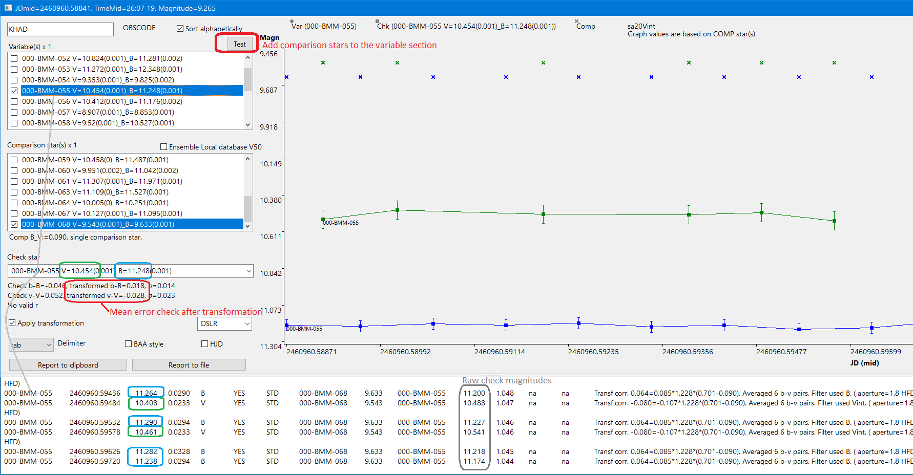
Testing your photometric measurements.
The AAVSO report window has a button "Test mode". If checked you can also select stable comparison stars with documented magnitudes as variable. This allows testing your measurements and comparing them with the documented B, V and R magnitudes of the selected comparison star. See also check your transformation error
Below is an example of the available variables in one image:
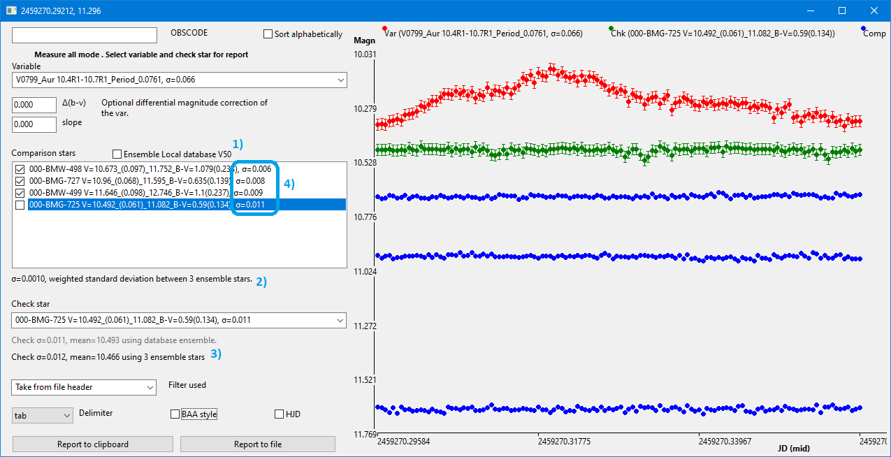
- You can switch between an ensemble of comparison stars or a Gaia ensemble. For a Gaia ensemble the comparison Johnson-Cousins and Sloan magnitudes can be calculated from the Gaia G, RP and BP magnitudes as set in the Photometry tab. For each star the magnitude zero point, m0 is calculated from the documented magnitude and the measured flux. This m0 should be the same for each star. The magnitude of the stars is defined as m = m0 - 2.5. log(flux). The weighted mean magnitude zero point of the ensemble is m0_ensemble = ∑( (wi/ ∑wi).m0_i ) where wi are the weight factors. For the comparison stars the weight factor is the flux expected by the documented magnitude. For the Gaia ensemble the measured signal to noise value (SNR) is used as a weight factor to reduce the dependency on only a few stars. For the Gaia ensemble, the outliers are removed and only ensemble stars with an SNR higher than 30 are used.
- This indicates the standard deviation between the m0 (zero-magnitudes) of the comparison stars. It is calculated as σtotal = (∑ ((wi/∑wi)*(m0_mean - m0_i))2)0.5 for each image and then averaged. The weight factor is the expected flux by the documented magnitude.
- This indicates the
standard deviation of the check star measurements. This is an important indicator of
the quality of the measurementw.
The lower, the better. The value indicates the combined noise of the
ensemble and the check star. It can be influenced by selecting a good
check star and good comparison stars. The
measured noise at 3) is in principle σtotal=
(σ2check + σ2ensemble)0.5 The
ensemble noise will generally be lower than the individual comparison
stars, but the result depends on whether the star noise (standard
deviation) is dependent or independent.
For a standard deviation so noise calculation either subtraction or addition you have to combine the uncertainties quadratically. The reason that a star ensemble has a lower standard deviation than a single comparison star is that the signal is averaged. So the total noise of an ensemble of four equal stars would be σtotal= ( (0.25σ)2 + (0.25σ)2+ (0.25σ)2+ (0.25σ)2 )0.5 equals σ/2. This doesn't happen when you use the ensemble m0 value for measuring the check star. The standard deviation of the check measurement result is higher and equal to σtota l= (σ2check + σ2ensemble)0.5
The tolerances shown in the graph are 2.5σcheck
Annotations could contain the following extras:
- "[At
Max]" Indicates the variable is near its
brightest epoch (within 5% of the calculated cycle period).
Note: This feature only works with the online database, as it relies on epoch data unavailable offline.
Testing status: Preliminary—if the calculation aligns with observations, please report it. - "Bad!" Indicates saturation—the star’s brightness exceeds the detector’s limit, causing flux loss and invalid measurements.
- "#" Indicates the variable star lacks an AUID (AAVSOs Unique Identifier). To report observations, request an AUID from the AAVSO first.
A) Define Bayer pattern: The green sensitive pixels of a DSLR camera have a very similar response as a Johnson-V filter and can be reported as filter TG. So to use the green pixels only, it is required to extract the green sensitive pixels from the raw. The images should NOT be converted to colour by the de-mosaic routine. To allow extraction the green pixel it is required to define the correct de-mosaic pattern in ASTAP. Load a raw image in ASTAP and in the "Stack method" tab check the temporary option "convert OSC images to colour". Set the Bayer pattern to Auto or one of the other patterns and test the conversion to colour with button the "Test pattern". This is best done with a terrestial image to be sure. If the correct pattern is selected and the colours produced are correct, then deselect the option "convert OSC images to colour".
B) Star Database V50. Check if the V50 star database is selected in the "Alignment" tab. If it is not available, download the V50 and select it.
C) For maximum accuracy it is better to calibrate the images first with darks, flats & flat darks. This can be done using the "calibration only"option in the "stack method" tab and then executing the regular stack procedure.
D) The measured star flux is compared and calibrated with the star database. For most cases you should install the V50 star database containing the Johnson-V magnitudes. After stopping the cycle it is possible to measure any object using the mouse pointer.
From the up to 1000 calibration stars any outlier star is removed if it deviates more then 1.5 sigma from the median factor (Gaia_star_magn - log(flux). For the remaining stars the factors are averaged and used for flux calibration of the variable and check star.. So it is a different setup than usual, but there is never a lack of calibration stars.
Calculation:
VMAG = ( VMAGINS - CMAGINS) + CREFMAG
equals
VMAG = VMAGINS + (CREFMAG- CMAGINS)
For a 200 Gaia stars ensemble:
VMAG = VMAGINS + mean[ (CREFMAG1- CMAGINS1),
(CREFMAG2- CMAGINS2), (CREFMAG2- CMAGINS2). . . . . .
(CREFMAG200- CMAGINS200)]
Prior to the mean calculation the outliers of (CREFMAGx- CMAGINSx)
values are removed above 1.5 sigma. Sigma is calculated from the
"median absolute deviation".
Same for the reported KMAG:
KMAG= KMAGINS + mean[ (CREFMAG1-
CMAGINS1), (CREFMAG2- CMAGINS2), (CREFMAG2-
CMAGINS2)......(CREFMAG200- CMAGINS200)]
E) Alignment of the images is done using the astrometric (plate) solution. The astrometric solution is written to the original file header. You can refresh the photometric and astrometric calibration using the dedicated buttons for this.
F) The list contains three dates:
- Date/time (start) in YYYY-MM-DDTHH:MM:SS. This is date & time from the header keyword DATE-OBS. This is normally the universal time at the start of the exposure.
- JD (mid exposure) This is the Julian Day of the exposure midpoint. This time is calculated from the keyword DATE-OBS and half of the exposure time is added.
- HJD (helio) Heliocentric Julian Day at the exposure midpoint expressed in UTC. This is the event time as seen from the Sun centre, compensating for the maximum ± 500 seconds time difference depending on the positions of the Earth, the object outside the Solar system and Sun. For plotting purposes only the fraction is displayed.
For a series of images, the standard deviation of the measured star magnitudes is typical better then 0.02 magnitudes. The standard deviation of the Check star is used for error estimate if more then 4 images are selected. otherwise an estimate based on the Variable SNR values is used. The star flux values should be below saturation (65500) but reasonable high.
G) Note that it is beneficial to de-focus an image a little to prevent pixel saturation and spread the flux measurement over more pixels. It also allows longer exposure times. However the image should be reasonable focused to allow solving.
Filter Passband:
- CV (clear view
- V or G or TG (Johnson-V or Bayer filter green),
- B (Johnson-B)
- RC (Cousins-red)
- SI (Sloan i')
- SR (Sloan r')
- SG (Sloan g')
If for the "Gaia comp stars" the option the local star database is selected only Johnson-V and Johnson-B are available.
If for the "Gaia comp stars" the option "Online Gaia-->auto" is selected the comparison magnitude either Johnson-V, Johnson-B, Cousins-red or SI, SR,SG will be the calculated from the Gaia three colour bands BP, RP and G using the Gaia transformation formulas. Use in the AAVSO report menu an "ensemble" as comp star.
Measuring the magnitude of asteroids
It is possible to measure the magnitudes of moving minor planets/asteroids. To make it work you first have to add asteroid annotations to all files. Go to the viewer menu Tools, Batch processing and execute menu "Add asteroid and comet annotation" for all files. The asteroids will be added as annotations in the FITS header.
Then in photometry tab, select all files, and click on the first file to plot. If the asteroid is not visible, switch on in the viewer pull down menu, "View", "Annotations visible". Then click on the asteroid to place the Var purple marker on the asteroid. This should generate a log measurement "Lock on ...." Then click on two reference stars to place the purple markers Check and 3. Then click on the ⯈| button to cycle once through the images. The columns for the magnitudes should be filled slowly.
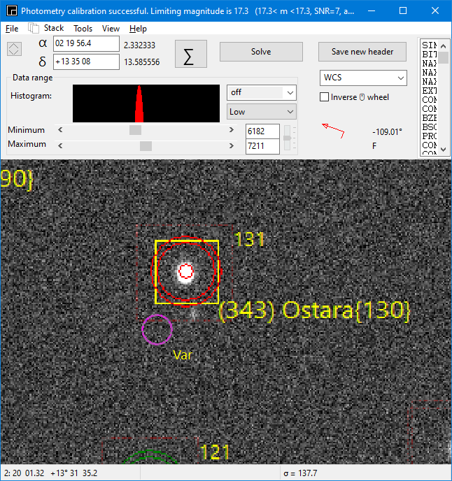
All command-line parameters are specified here
For ASTAP version 2026.04.11 or later:
Photometry can be executed by a command-line:
astap -p path
example
astap -p e:\temp\images
The directory could contain raw files. If check-mark option calibration is activated then it will first calibrate the lights and then automatically split them in TB, TG, TB frames.
Essential is to have an .ini file in this directory created by an earlier photometric report. Any AAVSO report generation will also write the setting to an .ini file. This file can re-used for next image series by placing it in the same directory as the new files.
The .ini contains will look like this:
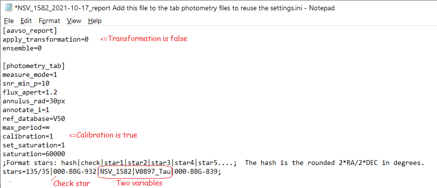
Inspector tab.
This tab is intended to measure accurately the tilt and curvature of your telescope & camera setup. It is done by calculating the best focus position for each image area. To do this it requires a series of images taken at several focuser positions. The routine will calculate from these images the best focus point of each area. It will measure the median HFD values of each image and area and build a table of HFD as function of the focuser position. From this data, curve fitting will give the transfer function and the best focus position expressed in focuser steps. The focus point differences between the image areas will indicate the tilt of each area. The difference between the centre and outer areas focus point will indicate the curvature.
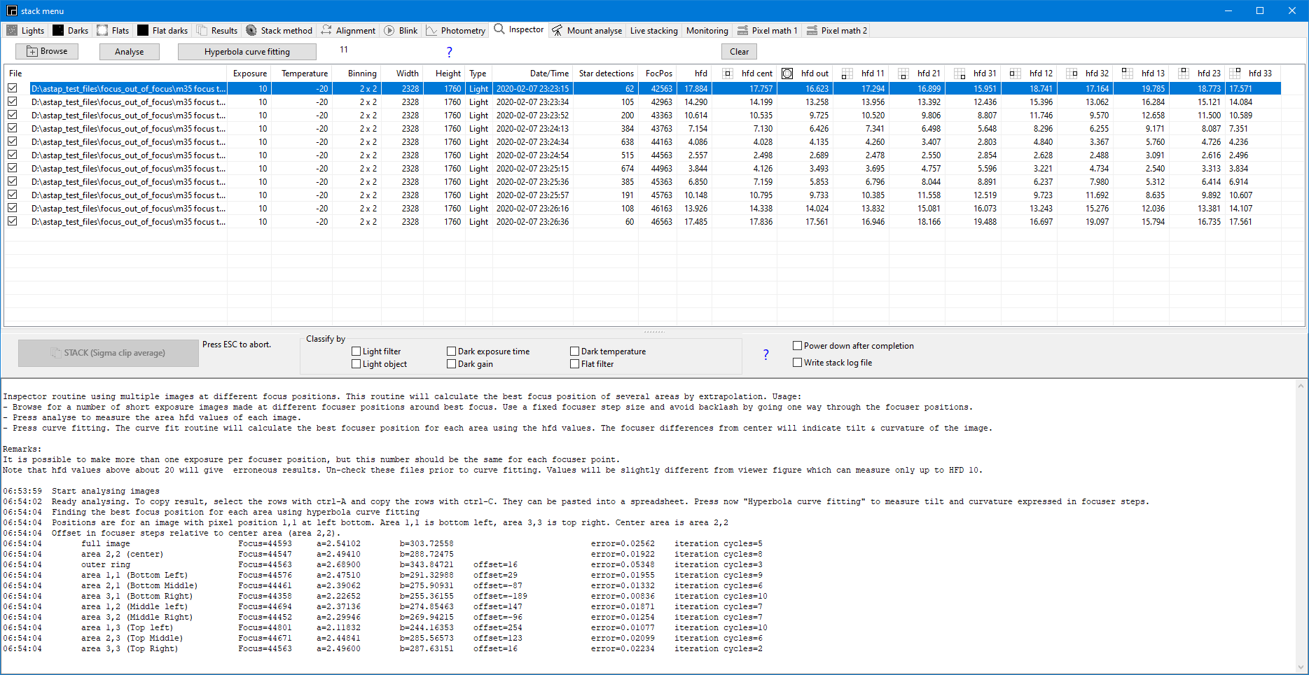
The usage is as follows:
- Prepare a series of short exposure images with different focuser positions and a lot of stars. Set the exposure time to a few seconds. Move for each image the focuser a small fixed step but only in one direction to prevent backlash problems. Images with stars having an HFD above 20 will not be analysed correctly.
- Browse with ASTAP inspector tab to the images.
- Press curve fitting.
- The difference between the focus point of each image area will be reported in focuser steps.
The reported HFD values can be selected and copied for further analysis in a spreadsheet.
The image areas "HFD centre" 2B (purple) and "HFD out" (any star at more than 75% from centre) are defined as followed:
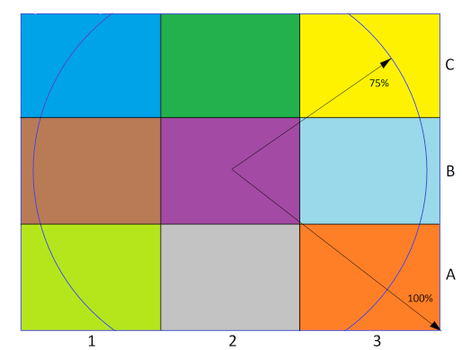
In addition the HFD values of the other eight areas are reported.
Back to index
This tab is intended to study:
- Mount pointing accuracy
- Polar alignment error
- Pier stability.
Mount pointing
accuracy:
take several images at different locations in the sky. Load the images
in the tab. Click on the button to add the
astrometric solutions. Click on the button analyse. To
analyse the result in a spreadsheet, select all
rows (ctrl+A), copy (ctrl+C) and paste them into a spreadsheet for
further
analysis.
Pier stability: Stop tracking of the mount and take images for several hours from a fixed position in the sky. Click on the button to add the astrometric solutions. Click on the button analyse. When the stability is perfect the azimuth (A Jnow [°]) and altitude (h Jnow [°]) should be stable within one arcsecond or less. Perfect stability is likely only to be achieved by a telescope mounted directly to a stable pier or wall. To analyse the result in a spreadsheet, select all rows (ctrl+A), copy (ctrl+C) and paste them into a spreadsheet for further analysis.
The images shall be in FITS or Astro-TIFF format with the mount α, δ position in the header. This is normally the case. Keywords required RA, DEC or OBJCTRA, OBJCTDEC.
The solution can be written
either in the original FITS file or in a separate .wcss file.
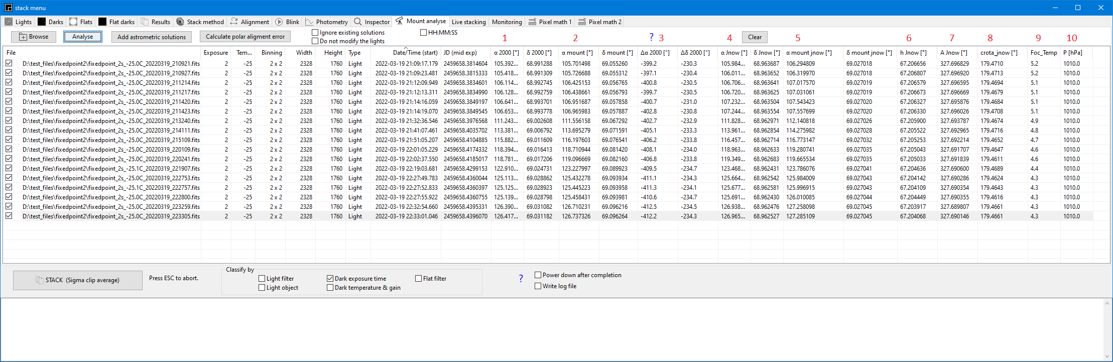
1) Image central position in equinox J2000
2) Mount position in equinox J2000
3) Difference between mount and image position in arc seconds.
4) Image apparent central position in equinox Jnow. The position is corrected for annual aberration and nutation but not for refraction.
5) Mount apparent position in equinox Jnow. The position is corrected for annual aberration and nutation but not for refraction.
6) Altitude of the image central position. The position is corrected for annual aberration and nutation and refraction.
7) Azimuth of the image central position. The position is corrected for annual aberration and nutation and refraction.
8) Rotation of the image for Jnow. This is the angle relative to a vector pointing to the Jnow celestial pole.
9) Focuser or ambient temperature. Used for the refraction calculation.
10) Atmospheric pressure in hPa/mBar used for refraction calculation. FITS header keyword shall be PRESSURE or AOCBAROM. For any different keyword, rename them to PRESSURE using the pop-up menu.
All file(s) in the specified directory will be stacked live. When it it is finished it will wait for new file(s). If a file is detected which is 0.2° away from the previous files a new stack will be started automatically. You can save the stack results from the viewer menu .
To identify files which are processed , they are renamed to the extension *.fts. You can rename them back with the button at the bottom.
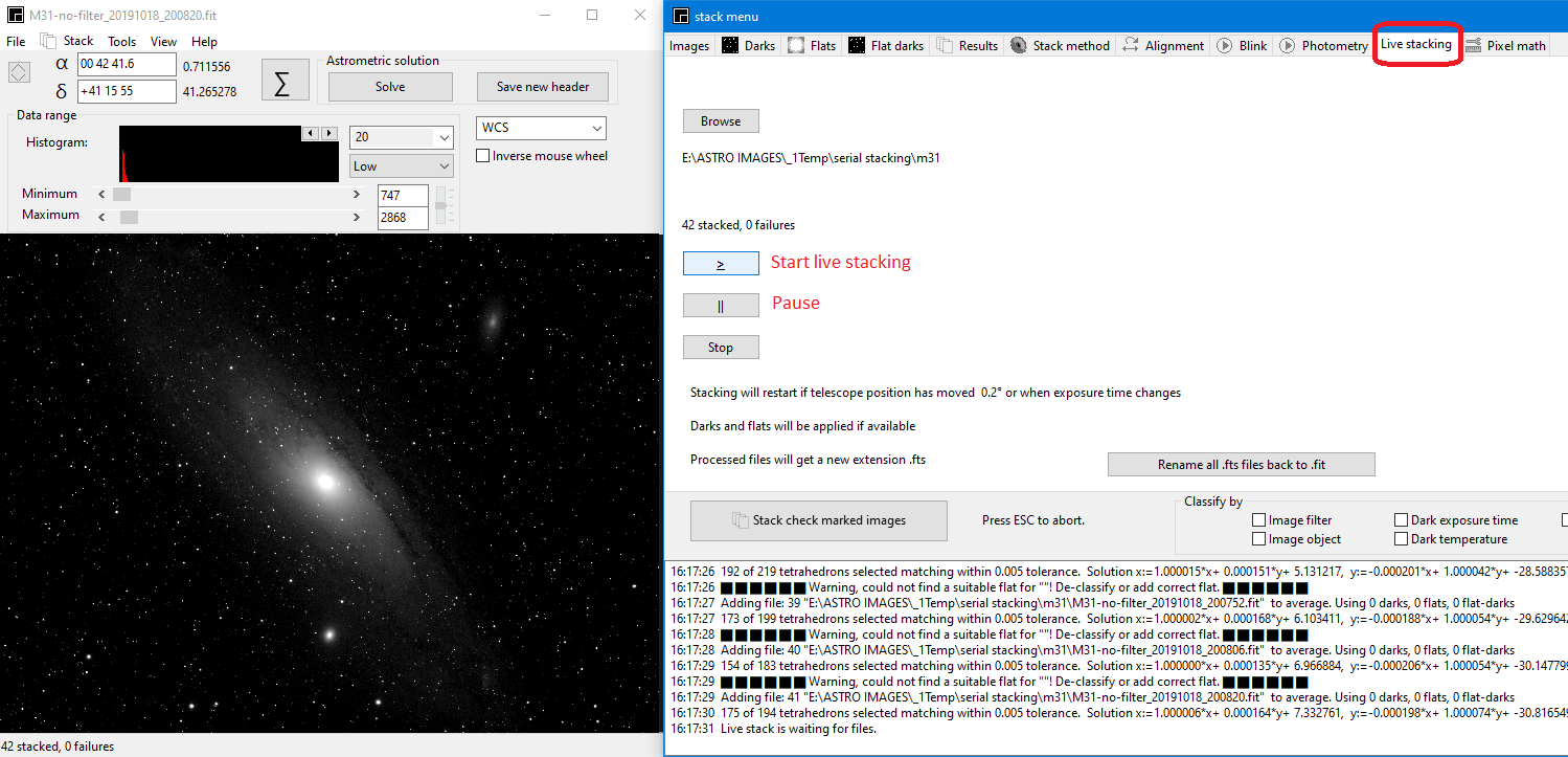
Note there is no rejection of poor images. All images are added with equal influence:
Assuming the images are A,B,C,D, E... then
Simple serial stacking:
result1:=A
result2:=(result1+B )/2
result3:=(result2*2+C)/3
result4:=(result3*3+D)/4
result5:=(result4*4+E)/5
Back to index
With this tab it is possible to monitor a specific directory for any new file. Any new file will be loaded in the viewer. After loading an optional action like "Tilt & HFD measurement" and "Solve image" can be executed. You could use this tab for monitoring the tilt adjustment progress or focus drift while taking images.
The action "Solve image" could be a useful option for users with a basic mount without encoders and a camera mounted on the telescope. An acquisition program like CCDCiel, Nina or APT can take continuous images with an exposure time of a few seconds. The saved images will be automatically loaded in the ASTAP viewer and solved. If a target or a position is specified the following information will be displayed.
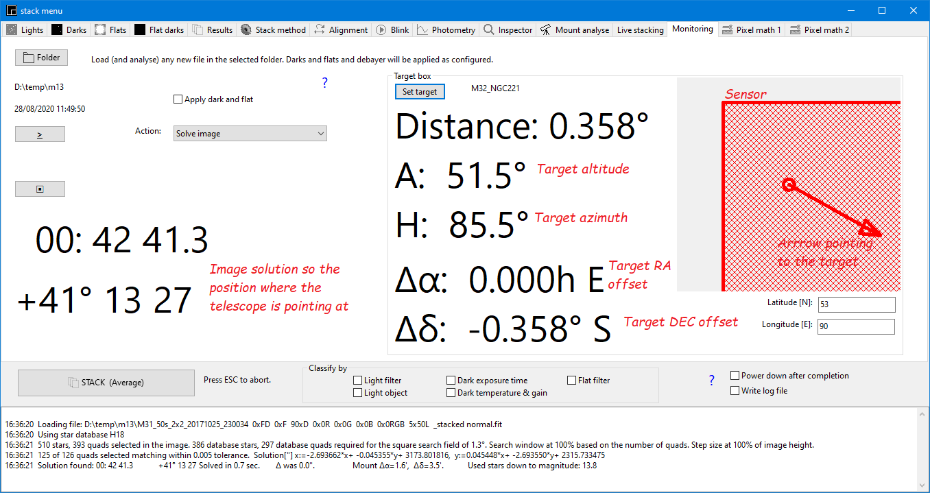
The sensor and arrow indicators are oriented for the azimuth & altitude. So up/down are in altitude. Left, right are in azimuth.
In the ASTAP viewer the user
can select under menu View an additional α, δ grid or
constellations overlay.
Several options including background equalising.
![]()
Powerful tool to remove a gradient. Follow steps 1 to 6.
For step 2) pull a rectangle around deep-sky objects/bright stars and select mouse pop-up menu "Remove deep-sky object (Oval shape) This will remove the object, allowing to create a smooth background. This background will be subtracted from the original image.
Step 6) will save the image
with a new file name ending with "equalised" . The same as 1)
and needs to be overwritten.
![]()
This is the test area for "satellite streak detection" It will be used in tab lights for "Analyse and organise images +" to display the number of satellite streaks in each image. It has three settings:
Gaussian blur: This is a blur which is applied for contour tracing. Typically set at 1.
σ factor: This is the sensitivity factor of the detection. The pixels which are this factor above the background noise are seen as signal. A typical value is 2. A lower value will make it more sensitive. A higher value is less sensitive.
Detection grid: This is the distance between the grid lines, the grid lines are used to minimise the number of pixels to test. Each streak will pass a horizontal or vertical grid line and full line detection will follow. By testing the grid only, the detection routine will be faster. Typical setting is 200 or 400 pixels grid spacing.
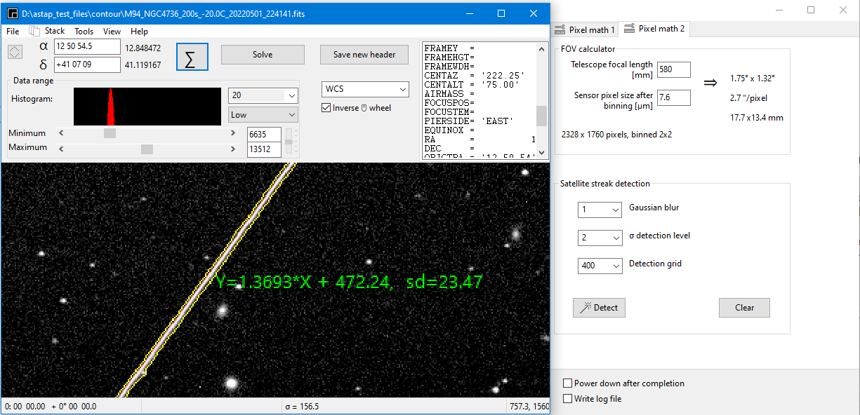
The reported noise indicated by letter σ is in ADU. The value can be reported in electrons (e-) by setting the option in the status bar pop-up menu. See other pop-up menus.
Viewer, reported angle
If the image the image is solved then the orientation will be reported by a north-east indicator. The reported angle is between the north arrow and the Y axis counterclockwise (rotate east from north) except when the image is flipped. For flipped images it is clockwise (rotate east of north). So for both flipped and unflipped images it is the angle reported between Y-axis and north arrow in the direction north to east.
A flipped image doesn't represent nature. The flipping (either horizontal or vertical) is caused by the camera system and will change the position of the north arrow. Nature has not changed so to report the correct angle the image has to be unflipped first. You can either unflip it vertical or horizontal but ASTAP is standard unflipping horizontal.
The same angle is reported in the header as keyword CROTA2. So the angle for flipped images is reported as if the image is "unflipped horizontal".
The reported angle is the rotation from sky to image orientation counter clockwise. The camera for taking the image was rotated with the same angle clockwise.
Header values:
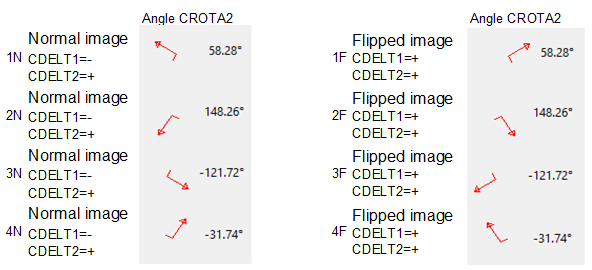
Note about the header: Old style solution keyword CDELT2 is always kept positive and if not the solution is flipped by negating both CDELT2, CDELT2 and shifting the angle 180 degrees. So if the image is flipped the solution is reporting "flipped horizontal" and not an equivalent "flipped vertical". The old style solution is in principle replaced by CD keywords.
To get a rotation angle for a flipped image, programmers could do the following:
if CDELT1*CDELT2>0 then
rotation:=-CROTA2 //flipped image
else
rotation:=CROTA2
or
if CD1_1*CD2_2 - CD1_2*CD2_1>0 then
rotation:=-CROTA2 //flipped image
else
rotation:=CROTA2
or
if (cd1_1*cd2_2-cd1_2*cd2_1)>=0 then sign:=+1 else sign:=-1;
rotation:= -arctan2(cd2_1,sign*cd1_1)*180/pi;//arctan2 returns arctangent of (y/x)
Rotation of camera is reported as follows:
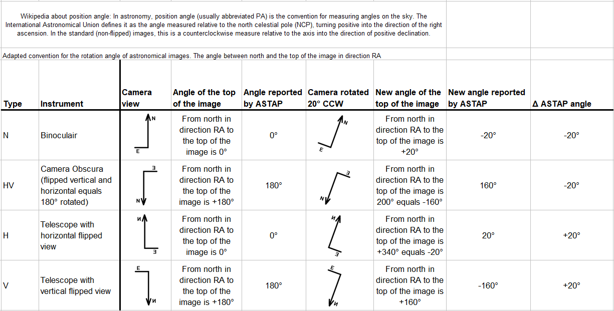
Back to index
If the program is associated with FITS image files or any other format, it will show the image as you click image file. Only one instance of ASTAP will be allowed. After clicking on the second image it will be shown in the first instance of ASTAP. If you want to open a second instance, just start ASTAP. If the program is started without parameters, you can open more instances.
Images can be loaded from the file menu or can be dragged and dropped on the main form.
Besides all FITS formats, the viewer supports most image formats in 8/24 bit or 16/48 bit format. It can export to any FITS format and 16/48 bit PNG and TIFF formats.
ASTAP can display images and tables of MEF, multi-extension FITS. The images of MEF can be saved as a single image. The MEF tables can be copied into the clipboard and pasted to a spreadsheet. (v0.9.446)
This ASTAP version can import raw images from almost any digital camera. For this ASTAP executes a modified Libraw tool "unprocessed_raw" which is included with the ASTAP for most editions. This special version exports directly to FITS including date&time, Bayer pattern and active areas of the sensor only. If "unprocessed_raw" is not included it can be installed in Linux by the "sudo apt-get install libraw-bin" command.
| File formats ASTAP | 8 bit | 16 bit | 32 bit (float) |
| Import | FITS, JPEG, PNG, TIFF, XISF (uncompressed) | FITS, FITS.FZ, PNG, TIFF (ASTRO-TIFF), PPM, PGM, raw formats, XISF (uncompressed) | FITS, FITS.FZ, TIFF (ASTRO-TIFF), PFM, XISF (uncompressed) |
| Export | FITS, JPEG, PNG, TIFF | FITS, FITS.FZ, PNG, TIFF (ASTRO-TIFF), PPM, PGM | FITS, TIFF, (ASTRO-TIFF), PFM |
From version 2026.07.16, ASTAP natively supports fits rice compressed files with extension fits.fz. GZIP compression is not supported.
The viewer has a preview function. After opening select "Preview FITS files". The preview is displayed in the ASTAP viewer. Use the arrow keys to move up or down or just click on the image. The current zoom and position are maintained so you could study the corner of a series of images on image quality.
The file open menu with preview selected:
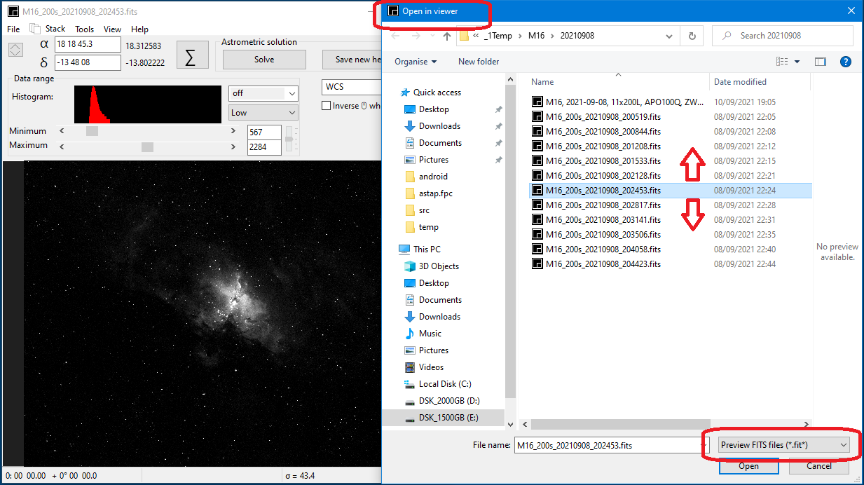
Back to index
Viewer, file menu, thumbnail viewer for FITS files
ASTAP has a FITS thumbnail viewer (ctrl-T). This could be useful to browse your FITS files. By clicking on the thumbnail it will be opened in the viewer. With a right mouse button click some options are available as changing directory, copy, move, rename or rename to *.bak.
The thumbnail size is dependent on the form size. Make it larger, the thumbnails will follow. Thumbnails are organized in 3*X. So the thumbnails are pretty big by purpose. The images are fully loaded in memory so it will consume some memory and time. So don't try to get thumbnails of 400 images.
Back to index
ASTAP viewer screen shot:
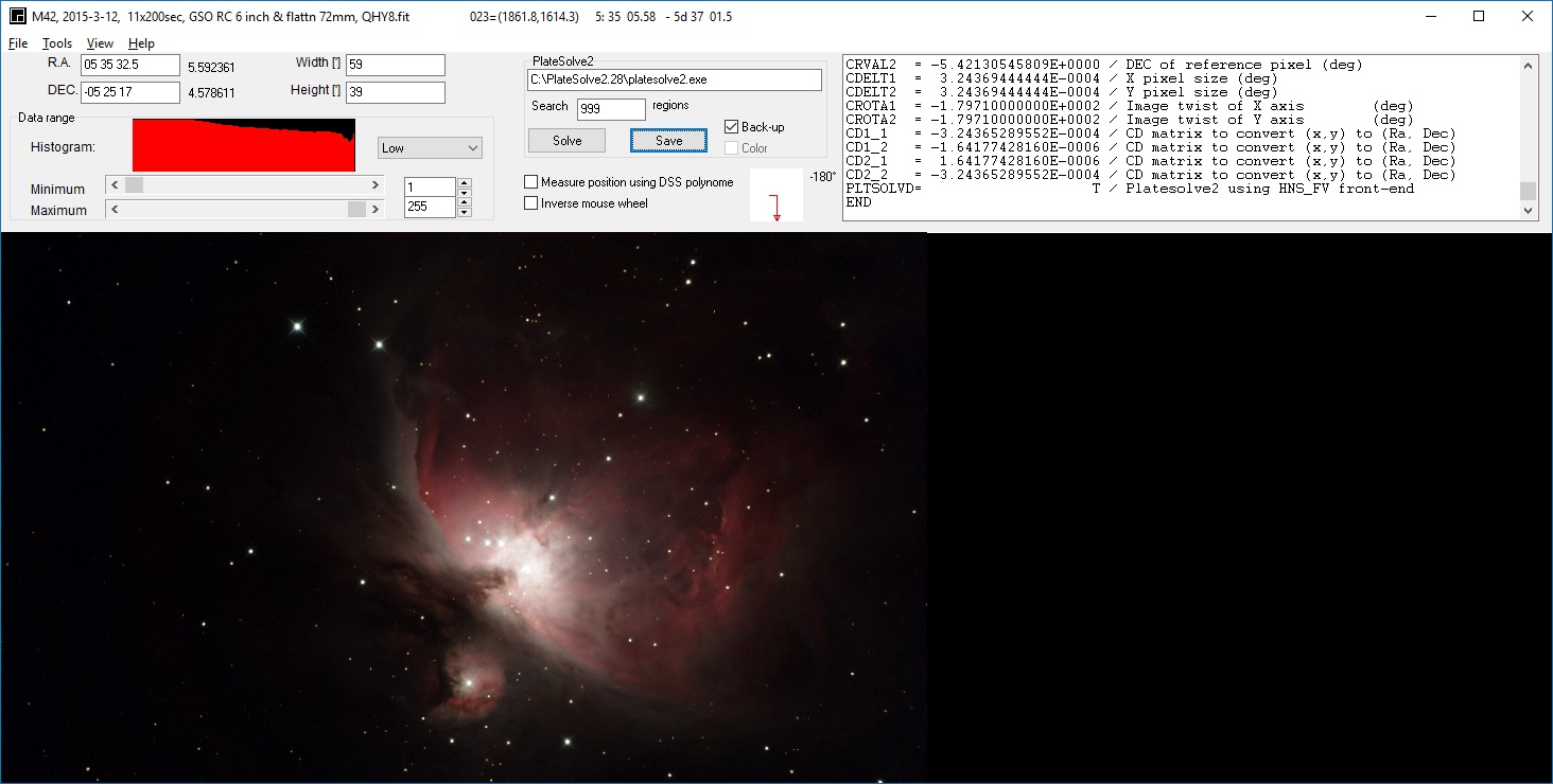
Viewer menu Tools:
Viewer, tools, Astrometric solving the image in the viewer
With the Solve| button it is possible to find an astrometric solution of the image loaded. For this the estimated celestial centre position α, δ should be available. This position is normally retrieved from the FITS header. Secondly the estimated image height in degrees should be specified in the stack menu, tab alignment. In the same tab alignment you can specify the search radius and down sampling. For successful solving see conditions required for solving.
For solving JPG, PNG or RAW files it is possible to add the object position as centre position using the deep sky database. Double click on the δ position in viewer and enter the object name. The position will be retrieved from the database. This position will be used as a start point for the solver.
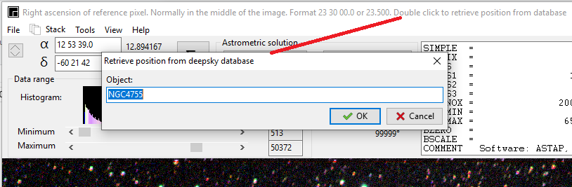
Back to index
Viewer, Tools, Batch processing:
With the batch routine several FITS images can be "astrometric solved" or converted. This conversion is not required for ASTAP. Automatic conversion is integrated in the menus.
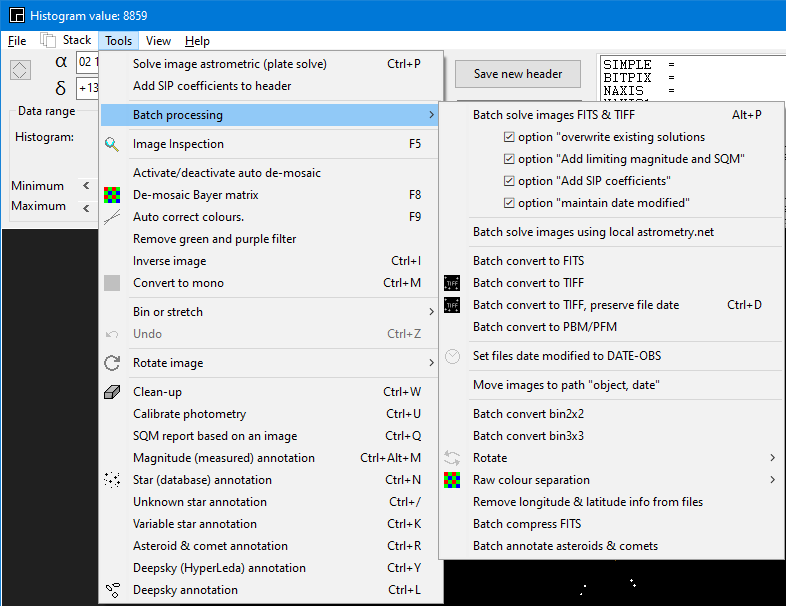
The functions "Batch solve FITS & TIFF" images and "Batch measure tilt and store to header keyword TILT" allow adding new values to the header. These can be reported in tab lights by setting the configurable last column to the desired header keyword. Once the images tab Lights are analysed then the data can be selected & copied and pasted to a spreadsheet for further use.
Back to index
Viewer, tools, Image inspection
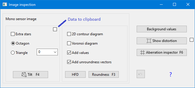
This menu is directly accessibly by F5. The tilt button can be activated by F4. It will show default an octagon based on the median HFD values of the stars in nine areas of the image. This will visualise any problem in the imaging system like sensor tilt and curvature. There are some other inspection options available like roundness (F3) and aberration inspector (F6).
The image used for testing should be a single raw image with sufficient stars and not containing a disturbing large and bright deep sky object. The exposure length should be long enough to image many stars but not too long avoiding star saturation.
The routine will detect and annotate the stars with their measured HFD value and plot a tilt indicator in the image. A star rich image containing a few hunderd stars or more gives the best accuracy.
The following will be reported:
- Image median HFD which is an excellent indicator of the quality of focusing. The lower the value the better the focusing, the sharper the stars are. The value is also dependent on the astronomical seeing and the quality of the optics. If the image is solved it will also be indicated in arc seconds.
- Sensor tilt as the
HFD difference between the best and worst corner median values. In
addition as an graphical indication it draws an trapezium in the image
based on the four median values.
There can be some variation in images of the same series. Any tilt equal or less than 10% of the range is a good value. Any tilt equal or more than 20% of the range indicates a tilt problem. - Off-axis aberration as the delta between the HFD value in the centre area and in the outer areas of the image. The stars in the outer area are normally a little larger, oval or comet-shaped due to the optics or curvature giving an higher HFD value. The lower this value the better the optics. This value could be a help to adjust the optimal distance between the field flattener and the camera. This measurement is only a valid if the focus for the centre area is perfect. A more advanced measuring method is available in tab CCD Inspector.
It is possible to automate the loading and tilt measurement using tab monitoring
An irregular octagon figure is displayed using the median HFD value of eight areas. If your optics is good and there is hardly any tilt or curvature the figure will form a square:. The yellow values indicate the median HFD values of nine square areas:
The figure of a good optical system:
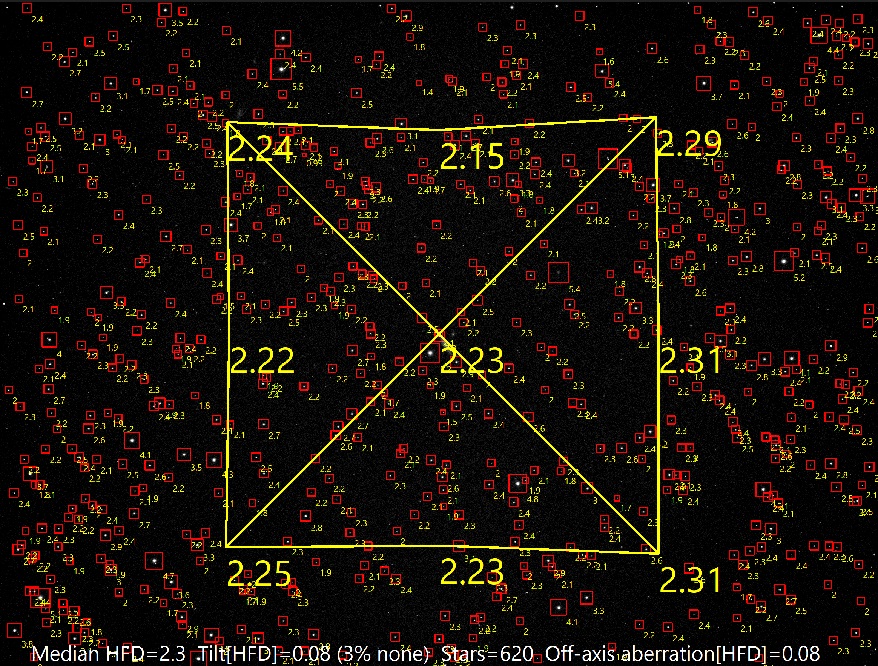
A system suffering from severe curvature:
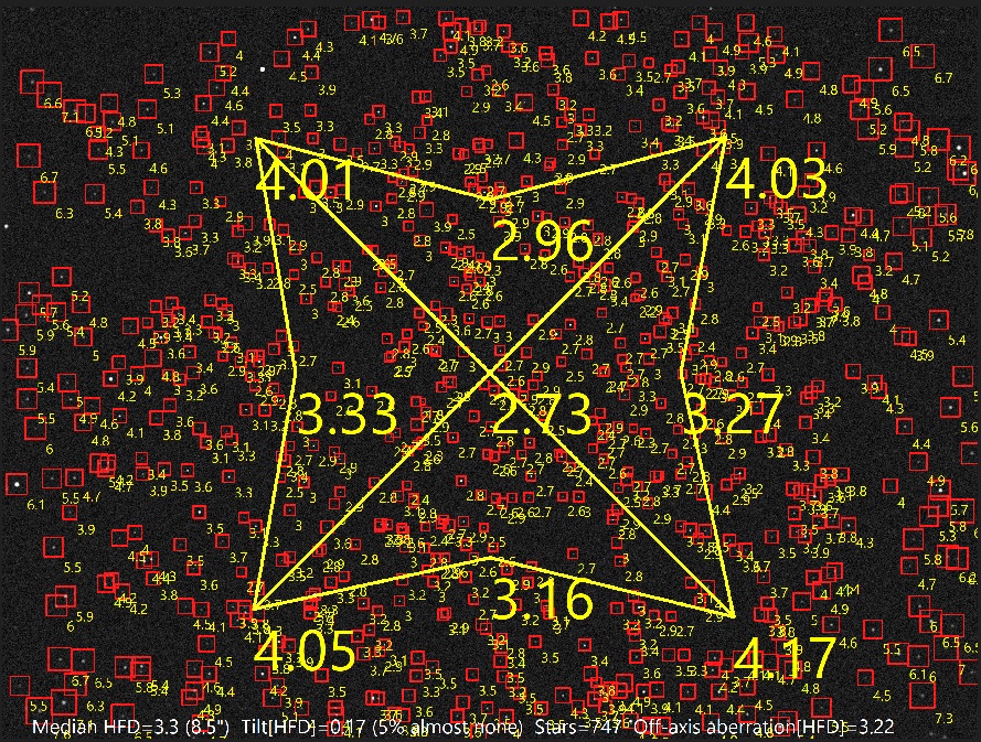
A system with severe tilt:
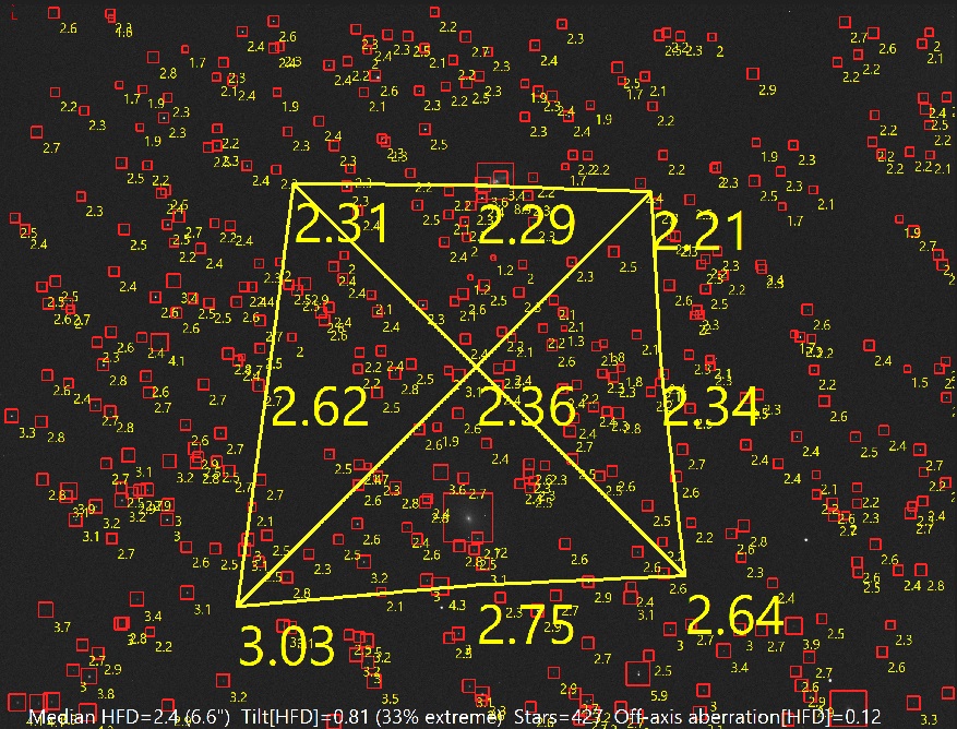
It is possible to automate the loading and tilt measurement using tab monitoring
CCD inspector calculation method explained:
HFDcentre = median(HFDarea 2B)
The OFF axis aberration = HFD_out - HFD_centre
The tilt is calculated as follows:
HFDworst = max(HFDarea 1A, HFDarea 3A, HFDarea 1C, HFDarea 3C)
Tilt [HFD] = HFDworst - HFDbest (of the corners)
Tilt [%] = 100% * (HFDworst - HFDbest ) / HFDmedian (note that the percentage scale is more dependent on focus)
The tilt scale is defined as follows:
None (0 to 5% tilt)
Almost none (5 to 10% tilt)
Mild (10 to 15% tilt)
Moderate (15 to 20% tilt)
Extreme (>30% tilt)
Triangle: The triangle based tilt indication is intended for adjusting your tilt adapter with three adjustment screws. First solve an image, then flip the image in the viewer such that north is up and east is left (northern hemisphere). Then apply the adjustable three corner angle such that the orientation of the adapter screw matches with the three corners shown. You can click on the tilt button without refresh.
The triangle based tilt indication is based on the following three areas:
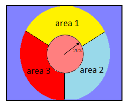
The triangle option measures in an circular area with a diameter equals the image height. This area is split in three equal 120 degrees segments. The centre is excluded.
It is possible to automate the loading and tilt measurement using live stacking
For the triangle the off-axis aberration calculation is as follows:
HFD_centre = median HFD value of all stars within 25% from centre.
The OFF axis aberration = HFD_out - HFD_centre
The tilt calculation:
Worst HFD value = max(HFD area 1, HFD area 2, HFD area 3)
Tilt = "Worst_HFD value" minus "Best HFD value"
The diameters of the areas 1,2 and 3 are equal to the distance to the longest side of the image. The triangle option is less sensitive than the octagon method but the areas are symmetrical so the orientation can be adapted without changing the sensitivity.
Normally the tilt indication uses stars with a signal to noise ratio (SNR) of 30 or higher. For extra stars it will reduce the minimum SNR to 10. Then the HFD values will be a little less accurate. Extra stars is intended for short exposure only where there are not enough stars with a SNR of 30 or higher.
Data export
If the option "data to clipboard" is checked then all available data is copied to the clipboard. If the image is solved the α, δ positions will be included. If the photometric calibration is applied it will include the star magnitudes.
An example of the data copied to the clipboard:
fitsX fitsY HFD RA[°] DEC[°] ADU Magnitude
1877.70 17.97 3.843 274.093663 -14.400684 229858 13.424
267.96 19.45 3.472 275.332120 -14.498080 141018 13.955
1172.71 18.24 3.040 274.635894 -14.444421 71522 14.692
2161.77 18.96 3.548 273.875327 -14.381897 167485 13.768
222.94 19.92 3.075 275.366797 -14.500390 218724 13.478
785.63 21.10 3.047 274.933882 -14.465880 169184 13.757
1392.94 22.41 3.522 274.466757 -14.427718 135043 14.002
2065.31 22.09 3.350 273.949687 -14.385719 87597 14.472
Back to index
HFD 2D contour.
The star half flux diameters (HFD's) are displayed in a 2D contour. Dark areas indicate lower and therefore better HFD values. This will quickly visualise sensor tilt or other problems. To avoid false indications by outliers the HFD values are filtered by taking the median HFD value of the three closest stars and allocating the result to all three stars. The HFD values are indicated numerically. The grey levels have no direct linear relation with the HFD.
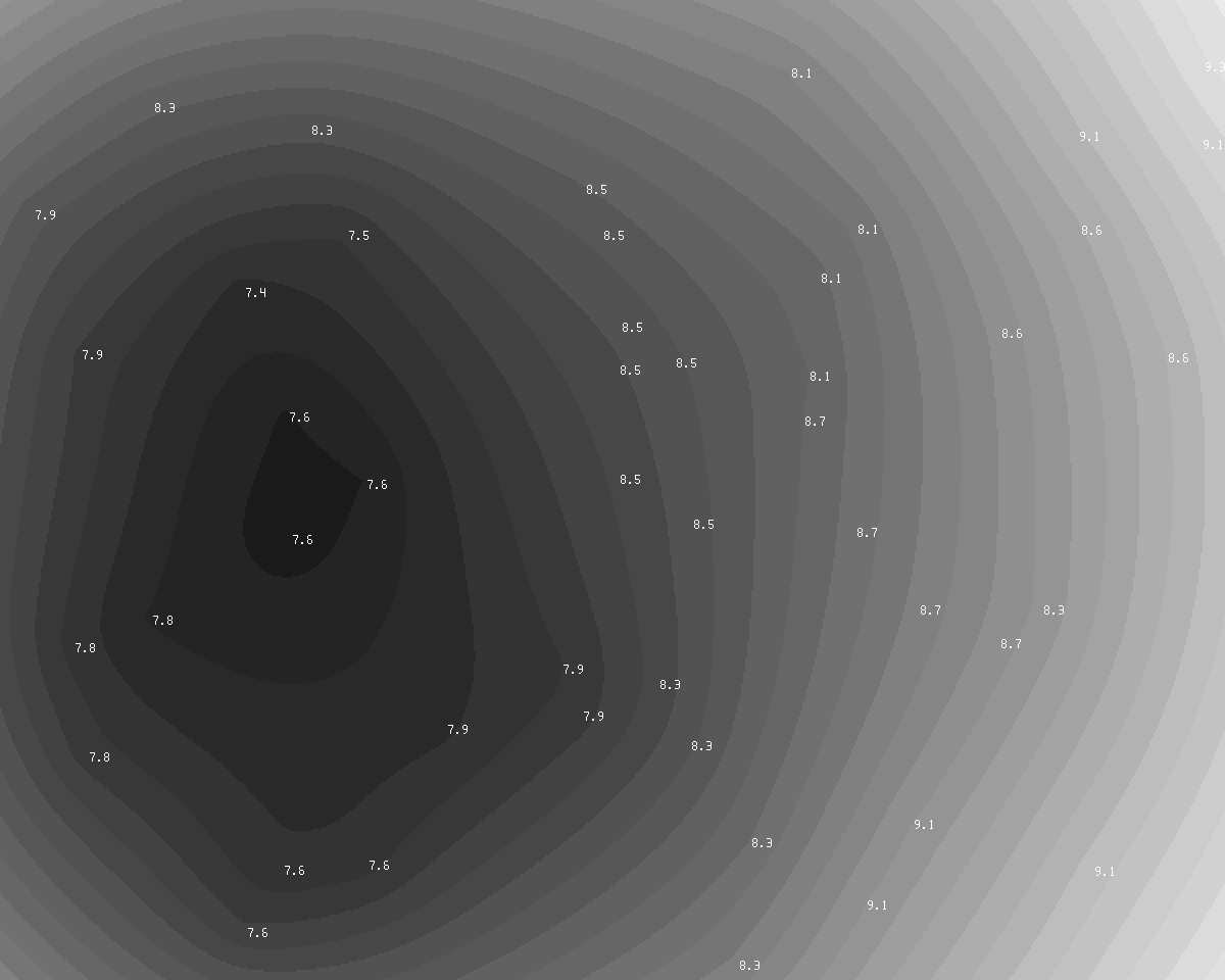
HFD diagram.
The star HFD values can also be represented by areas of constant HFD. It is in principle a Voronoi diagram, but by taking the median value of the three closest stars and allocating the median to the three stars it looks a little different.Bright areas indicate a star with a high HFD value. Darker areas indicate a lower value. The grey level is the HFD * 100.
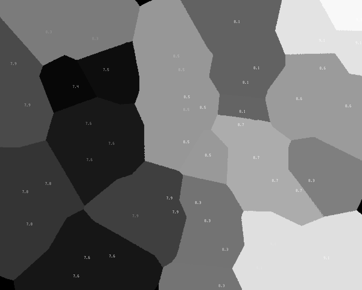
HFD values
This tool will only indicate the median filtered HFD values next to the stars. These are the same values as in the 2D contour and HFD diagram. To avoid false indications by outliers the HFD values are filtered by taking the median HFD value of the three closest stars and allocating the result to all three stars.
Unroundness
This tool measures the unroundness of the imaged stars. The values are the aspect ratio of an ellipse.
Measuring principle: The star is split in two by a line. The average distance of the pixels to the split is measured. Then the split line is rotated one degree and again the average pixel distance to the split line is measured. This continues untill the line has made a 180 degree rotation. The aspect ratio is the highest distance value found divided by the lowest distantce value. The orientation is the position where the lowest distance is found and the star is the longest.
This
unroundness measuring principle is licensed under a Creative
Commons Attribution 4.0 International License.
Median background values
This tool writes the median background values as numerical values in the image. Stars will be ignored but nebulae will influence the background measurement..
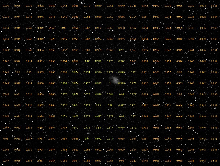
Show distortion
This tool shows the difference between the Gaia star positions and the centroids of the imaged stars, assuming a linear solution. A difference is indicated with a line 50x larger than the actual difference in pixels. A scale is show at the left bottom and the median astrometric error in arc seconds for the centre 50% square (height/2 * height/2) is reported. This indicates the error to expect for astrometric measurements. Note the database resolution is 0.077" in α and 0.039" in δ.
If the SIP polynomial is selected as measuring mode in the viewer then the distortion will be corrected for the reported values in the status bar.
Back to index
Aberration Inspector
This tool creates a 3x3 mosaic of the image's centre, the corners and borders. This allows an easy comparison of the star shape at the different sections of the image.
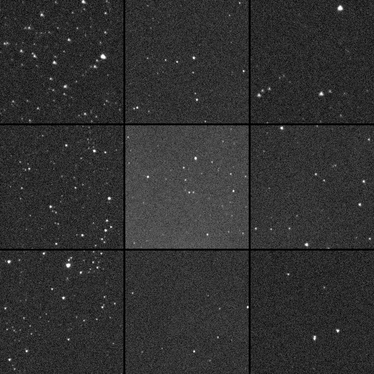
Back to index
Viewer, Tools, Calibrate Photometry.
With this option the relation between flux and magnitude is measured. The image should be solved in advance to be able to calibrate the star flux with star database magnitudes. After the calibration is applied, the star magnitude at the mouse cursor is displayed. In the log an estimate for the limiting magnitude for point sources is reported for a detection limit of SNR ≥7. The accuracy is better than ±,0.5 magnitudes. The aperture used for star flux measurement can be adapted in the stack menu tab "photometry".
For stretched images the reported (limiting) magnitude will be less reliable. Use the pop-up menu option "online query" to request the magnitude of the point sources.
Viewer, Tools, SQM report based on an image
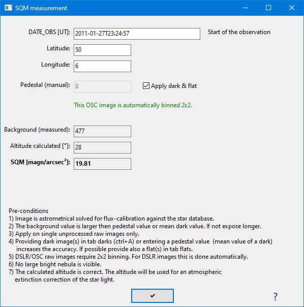
With this option the SQM = sky background value relative to the stars is measured and expressed in magnitude per square arc second. The image should be solved in advance to be able to calibrate the measured star flux with star database magnitudes. The reported SQM value will be equal to a value reported by a Unihedron SQM-L meter. Atmospheric extinction of the stars at lower altitudes will be compensated.
Some background information:
http://www.lightpollution.it/download/sqmreport.pdf
At zenith the measured star flux and sky background flux are defined as comparable and star light extinction is zeroed by subtracting 0.28 magnitudes from the calculated zenith extinction. So at zenith the SQM brightness values are comparable to deep-sky object brightness and can be expressed in magn/arcsec². At lower altitudes the measured star flux is less and compensated by a predicted extinction (0.2811*airmass, airmass according to Pickering).
Pre-conditions
1) Image is astrometrically solved for star flux-calibration against the star database magnitudes.
2) The background value is larger than the pedestal value or mean dark value. If not expose longer.
3) Apply on single unprocessed raw images only.
4) Providing dark image(s) in "darks" tab (ctrl+A) or entering a pedestal value (mean value of a dark)
increases the accuracy. If possible provide also a flat(s) in "flats" tab.
5) DSLR/OSC raw images require 2x2 binning. For DSLR images this is done automatically.
6) Most of the image is free of deep-sky nebulae.
7) The calculated altitude is correct. The altitude will be used for an atmospheric
extinction correction of the star light.
8) No filter is used except a UV/IR block filter. (Note the standard database is based on the Gaia blue magnitudes (400-700 nm) which matches the passband of a typical camera. In case the V50 photometry database is selected, a matching Johnson-V filter should be used.)
Differences between Unihedron and ASTAP measurements:
- The Unihedron is an absolute measurement of the sky glow. The ASTAP measurement is relative to star light measurement. In case of poor sky transparency ASTAP will report lower SQM values due to the higher extinction of star light.
- It is expected that the ASTAP measurement will be less sensitive to Milky Way light since it measures the background and not the total sky glow.
- The Unihedron measurement will be less sensitive to the blue part of the spectrum.
Viewer, Tools, Magnitude (measured) annotation.
With this option the stars are annotated with the estimated magnitude. The image should be solved in advance to be able to calibrate the star flux with star database magnitudes.
If the Johnson-V version of the star database (V50) is used, the results match very accurately with AAVSO charts as demonstrated below. The camera was an ASI1600 with only an UV-IR block filter:

For best accuracy, the image should be monochrome and either the Gaia Johnson-V star database V50 should have been installed and selected or use the online access to Gaia (Simbad server). Gaia magnitudes retrieved online will be converted to Johnson-V or others depending on the filter name. The image should have been taken with a Johnson-V filter or none (clear). Saturated stars will be ignored since it is not possible to measure them accurately.
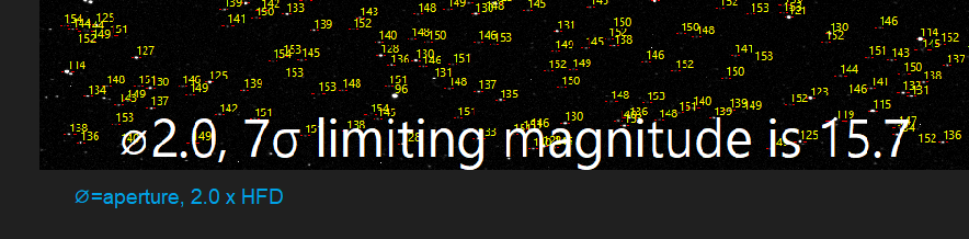
In the bottom left corner of the image an estimate for the limiting magnitude for point sources is reported using a detection limit SNR ≥ 7. Below this value detection of point sources becomes unreliable. The accuracy is better than ±,0.5 magnitudes. The image should not be stretched. The aperture used for star flux measurement can be adapted in the stack menu tab "photometry". Results can be validated by requesting the Gaia BP magnitude magnitude of the faintest stars in the image using the pop-up menu option "online query".
For stretched images the reported limiting magnitude will be less reliable. Use the pop-up menu option "online query" to request the magnitude of the faintest sources.
Back to index
Viewer, Tools, Star (database) magnitude.
With this option the stars are annotated with the star database magnitude. This can be done best with V50 containing the calculated Johnson-V magnitudes.
For a G-database the indicated magnitude is Gaia blue. For a V-database the indicated magnitude is Johnson-V and the following is the difference between Gaia blue and red, positive for reddish objects. All in 1/10 of a magnitude.
Below, the image is 1) solved, 2) auto calibrated (using the V16) . The cursor is at a star and based on the flux of all known stars, the star Johnson-V magnitude is estimated to be 16.1. The stars are marked with the Johnson-V magnitude and Bp-Rp color indication.
See also blink and photometry
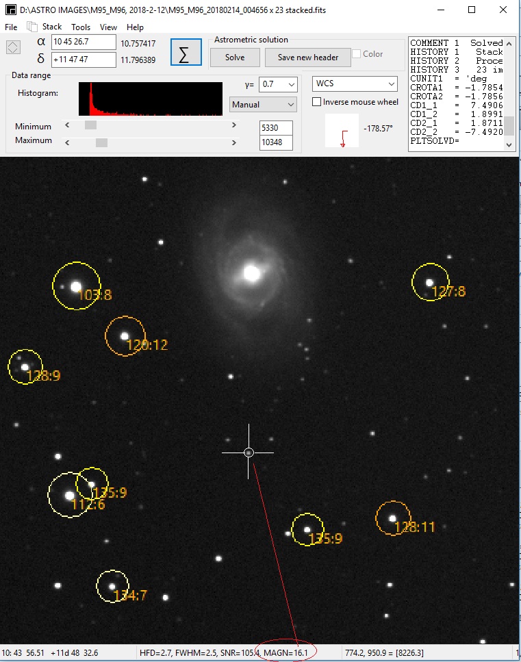
Back to index
Viewer, Tools, Unknown star annotation (nova detection)
Any unknown object or a star with an abnormal magnitude is identified. This option is intended to mark novae and minor planets using the star database. Any star like object missing or with one magnitude brighter than the online Gaia database is annotated. The Gaia online database goes down to about magnitude 21. So the algorithm will detect any new object to about 21-1 is magnitude 20. The image should be solved in advance.
Downloading the Gaia database could be slow. Especially for field-of-view larger than two degrees.
Novae inside small galaxy boundaries could avoid star detection. Very small galaxies could also be detected as missing in the Gaia star database for the obvious reasons. Any object which is not identified in the Gaia catalogue is annotated but objects thar are more spread out are labelled as clouds. This is typically the case for H-alpha clouds or galaxies.
Annotations are stored in the FITS header.
The same algorithm can be applied batch-wise using the popup menu of the lights tab processing.
Viewer, Tools, Variable star annotation
Variable stars are annotated using the variable_stars.csv database.
Viewer, Tools, Asteroid and comet annotation
This option will annotate asteroids using the orbital elements taken from the MPCORB.DAT file and for comets the ComeEls.txt from the Minor Planet Center.
Usage:
- Solve an image.
- Go to to the viewer "Tools" menu, "Asteroid annotation".
- First time download the full MPCORB.DAT from the minor planet center. The link is available from the blue down arrow. Set the path to MPCORB.DAT correctly.
- Set the limiting magnitude and maximum number of asteroids to read.
- Press the button Asteroid & comet annotation .
Remarks:
Renew the MPCORB.DAT and CometEls.txt files every few months.
The observation date and time are extracted from the FITS header (date-obs, date-avg) or for other files the file date is taken. If the date average is not available it will be calculated from the exposure time and date-obs from the FITS header.
The latitude and longitude of the observation location are also taken from the header. If not available enter them manually or leave them at 0.
For MPC1992 style reporting the option "Add as annotation to the FITS header" should be set.
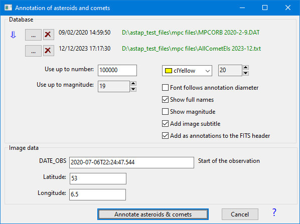
Back to index
Viewer, Tools, Deep sky annotations
If the image is solved, it is possible to add deep sky annotations. See pull-down menu TOOLS:
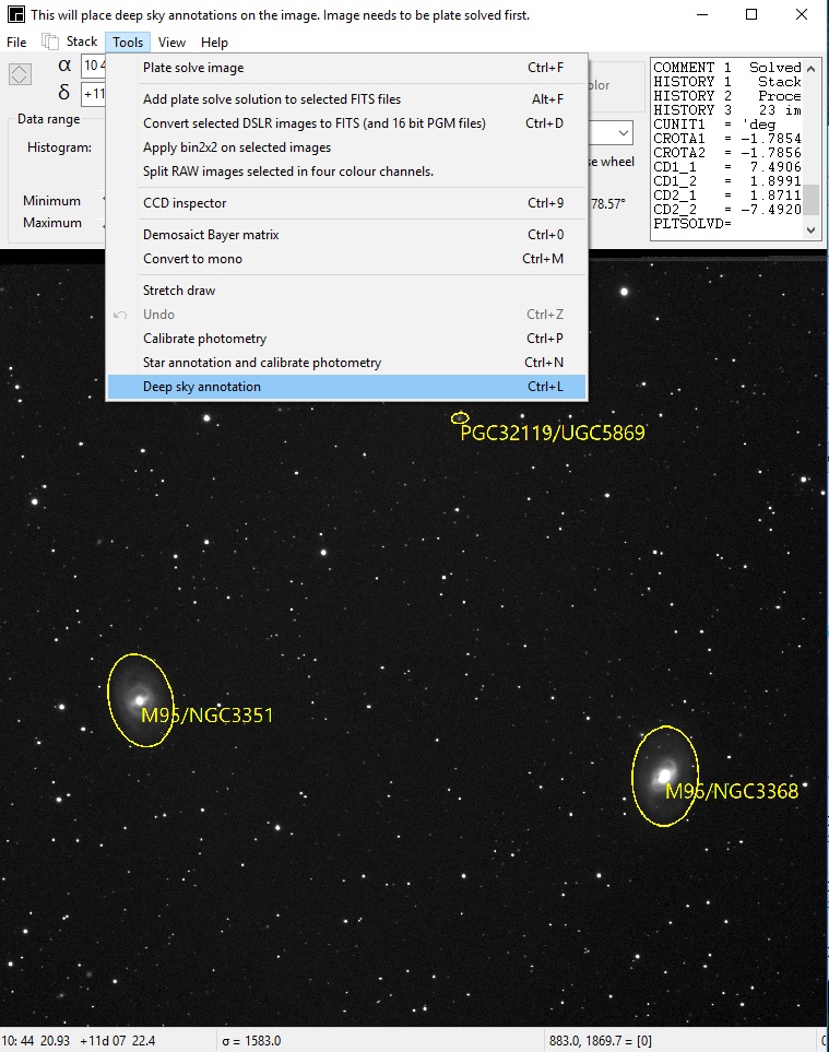
Back to index
View menu
This menu has the following options:
- Image clean up Ctrl+space
- Centre lost windows Ctrl+F12 Use this if you have multiple screens and once window is out of sight for some reason.
- Flip horizontal Ctrl+H
- Flip vertical Ctrl+H
- Zoom out PgUp
- Zoom in PgDn
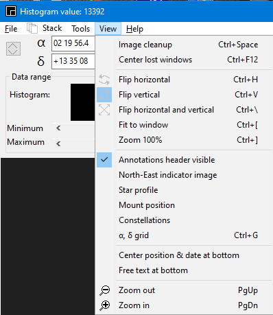
Back to index
FITS
tables
The
viewer has limited support for displaying FITS binary and ASCII tables.
It can read and write binary tables and read ASCII tables only. They
are displayed in the memo. Values are separated by a tab #9 and can be
selected and copied to a spreadsheet. It can display only one table and
will display the first table only. The file can be saved again but all
binary values will be all be written as 4 byte float.
Back
to index
Viewer pop-up menu:
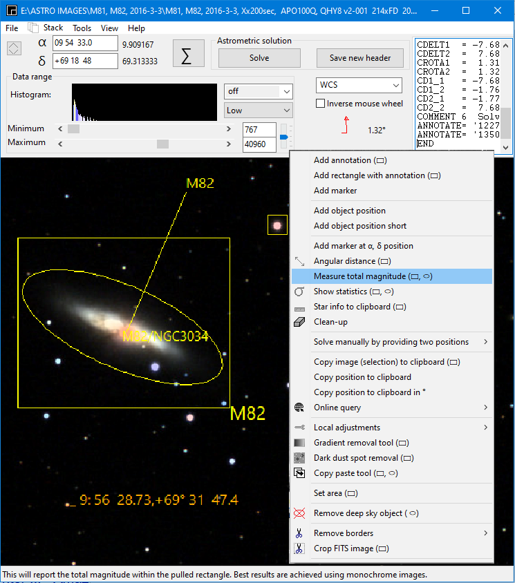
Add annotation: free text label at an x,y position. It can be connected via a line by first holding the right mouse button and moving the mouse away. See sample above. Persistent by annotation keyword in the FITS header. The annotation can be switched off in the pull-down menu "View". Remove by removing the annotation line in the header. If a @ is added to the text, the annotation is written persistently in the image data. So the image will be permanently altered after saving. Adding two or more @ will increase the font size.
Add marker: rectangle marker at x,y position. Draw the rectangle first by holding the right mouse button down and moving the mouse away. See sample above. Persistent by annotation keyword in the FITS header. The annotation can be switched off in the pull-down menu "View". Remove by removing the annotation line in the header.
Add object position: Enabled after astrometric solve. Will add the α, δ at the mouse position. Orange if a lock is possible, see above sample, red if not. Not persistent after image clean up.
Add marker at α, δ position: will place a yellow square at the specified α, δ position. See above sample for orange star. Enabled after astrometric solve. Persistent. Position will be saved with "save settings". If C is typed, the marker is placed at the centre.
Measure total magnitude within shape: Enabled after astrometric solve. The shape is either a rectangle or a ellipse is SHIFT or CNTRL is pressed. The program will measure the flux and try to estimate the magnitude. Hold the right mouse button down and pull a rectangle around the deep sky object, release mouse button and then select this menu. If the image is taken with a Johnson-V filter then also the V50 Johnson-V star or online star databases should be used. All other local database that are used for flux calibration are based on Gaia Bp. If more than 3% of the pixels are saturated a warning will be given.
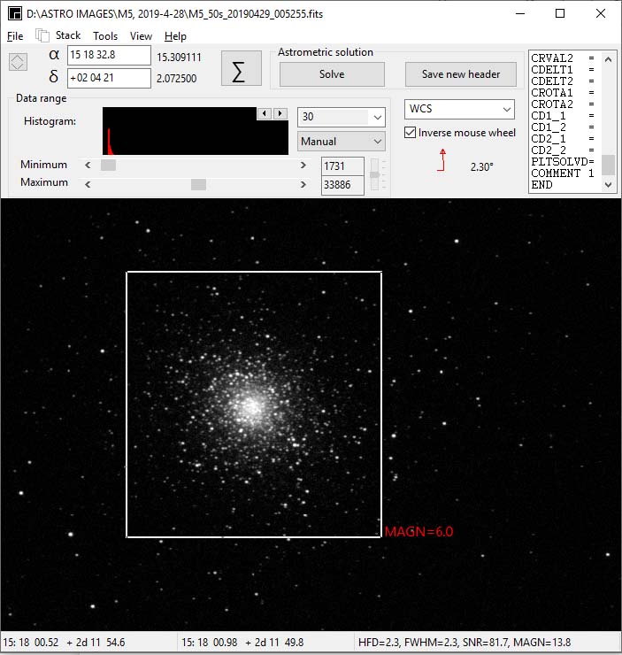
A demonstration is available on YouTube: Photometry in the viewer
The measuring principle is as follows:
- Use the star database to measure the MEDIAN relation between flux of the detected stars and star magnitude from the database. (That's why solving is required and best results are achieved with the V50 Johnson-V star databases based on Gaia DR3)
- Measure the MEDIAN background 1 to 10 pixels wide outside the rectangle box. This median measurement will ignore stars in the field.
- Measure the MEAN flux inside the box.
- Calculate the magnitude for the "inside mean flux" minus "median outside box flux" using the relation found for the stars.
You could argue that a Johnson-V filter or green channel is required for the image but in practice the error is limited depending on the spectrum.
MPC1992 report line: This menu will report the position of a minor planet at the mouse cursor to both the clipboard and the standard log. If the object is within an annotation the report will include the object abbreviation. To include abbreviations the annotations have to be added prior to using the MPC1992 report line. See viewer menu "Asteroids & comets annotation" shortcut ctrl+R.
Usage: Place the mouse pointer on an minor planet spot and select this menu. The minor planet name, position and magnitude will be reported both in the clpboard and the log. This works best in combination with the track and stack menu of the blink tab. The reported line can be pasted directly into the online MPC checker. No need to enter the date and position. Just paste the single line of 80 characters long. A MPC1992 report could be assembled manually with these lines to a full report. A report should contain typically three observations of one object in a single night.:
A MPC1992 template for reporting asteroid/minor-planet positions to the Minor planet Center
COD XXX
CON Optional contact
name. Additional contact details may then follow.
OBS Observer
name(s), no programs
MEA Measurers
name(s), no programs
TEL 0.2-m f/4
reflector + CCD
COM Long. 01 30 00
E, Lat. 53 00 00 N, Alt 10m, Google Earth
NET Gaia3
63343
B2018 09 10.54372 22 57 15.97 -07 38
51.9
19.76B XXX
38826
B2018 09 10.54372 22 56 42.42 -07 50
37.1
18.19B XXX
....
Show statistics:
This menu will generate a statistics report of the image.
Star info to clipboard: This will generate a positional and photometric report of all detectable stars in the selected window and place it in the clipboard. From there the information can be copied to your favourite program/spreadsheet. This menu will only be available if the image is solved. (Press viewer solve button). The magnitudes value are absolutely calibrated values based on the selected reference database.
The report in the clipboard will look like this:
Example of an ASTAP report:
Limiting magnitude is 18.1 (18.1< m <18.1, SNR=7, aperture ⌀1.5)Passband filter used: CV
Passband database=BP
fitsX fitsY HFD α[°] δ[°] ADU SNR Magn_measured | Gaia-V Gaia-B Gaia-R Gaia-SG Gaia-SR Gaia-SI Gaia-G Gaia-BP Gaia-RP
3755.45 2692.99 3.604 23.747631 30.448624 31952 118 14.797 | 14.620 15.480 14.134 15.003 14.347 14.103 14.380 14.828 13.766
3826.88 2702.46 3.386 23.778321 30.445076 6398 30 16.544 | 16.377 17.496 15.773 16.887 16.008 15.663 16.035 16.618 15.321
3803.23 2709.42 3.958 23.768154 30.442512 27335 110 14.967 | 14.793 15.309 14.473 14.987 14.662 14.548 14.668 14.949 14.225
3787.76 2712.94 3.378 23.761501 30.441217 8257 34 16.267 | 16.232 16.877 15.846 16.502 16.045 15.881 16.065 16.407 15.549
The values are separated by a tab. The reference database, aperture and annulus can be selected in tab photometry. For measuring the absolute magnitudes it will use the reference magnitudes of either a local star database (e.g. the D50, Gaia BP or the Johnson-V in the V50) or the online Gaia catalog from Vizier. About six photometric transformations are available for the Johnson V, B, R and Sloan magnitudes according to the transformation as documented in the Gaia documentation. The online Gaia reference data is retrieved from Vizier and the retrieval can be slow. The magnitude transformation is done locally.
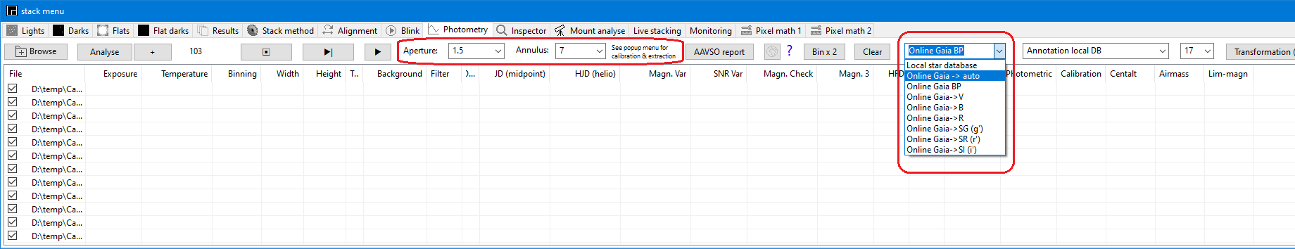
To measure all the stars in a series of images use the tab photometry and option "measure all stars in one step".
Copy image (selection) to the clipboard: copies the displayed image or a selection of the image to the clipboard. The orientation is depending on the selection direction.. So the image can be flipped both vertical and horizontal depending on the selection direction..
Copy position to the clipboard: Enabled after astrometric solve. Copies the α, δ position to the clipboard.
Copy position to the clipboard in ° : Enabled after astrometric solve. Copies the α, δ position in degrees to the clipboard.
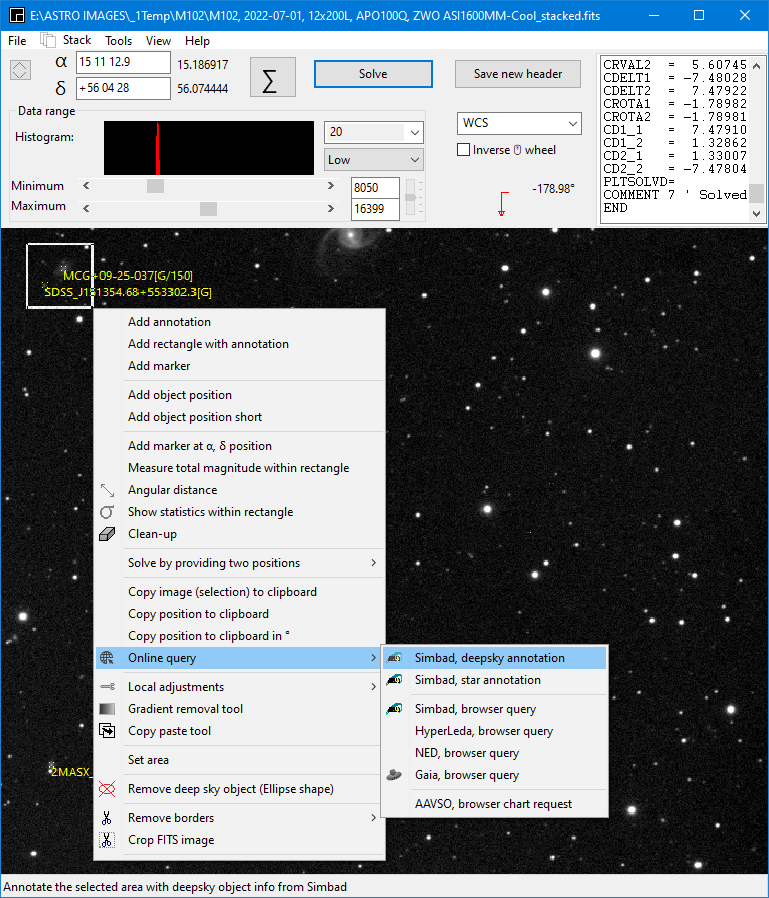
Online query: Query the Simbad database, Hyperleda, Ned or Gaia online database for all objects within the selected rectangle. Or request an AAVSO map for the selected rectangle. The annotation requests will annotate the objects in the image. The browser requests will activate the default web browser and list the objects found in a table with information and further links. For a Gaia query it is better to place the cursor directly on the star rather than pull a rectangle.
Local adjustments
Local remove colour.
Local Gaussian blur.
Local equalise tool.
Brighten a small area based on the corner values.
Gradient removal tool
To remove a linear gradient caused by light pollution or twilight. The routine needs two empty areas 40x40 pixels in the image to measure the gradient. The area may contain stars but no deep-sky object. The area is selected by pressing the right mouse button(first area) and while holding the mouse button move to the second area in the direction of the gradient. Then select the "Gradient removal tool" from the pop-up menu. Try to maximise the distance ideally to the full image range.
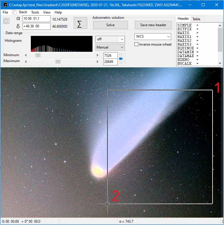
Dark spot removal tool: Tool to remove dark round spot by dust in the optical system, Hold the SHIFT or CTRL button and press the right mouse button to accurately encircle the dark spot. Release the right mouse button and select the "dark spot removal tool". For a demonstration see this Youtube video.
Copy paste tool: Powerful touch-up tool for cosmetic corrections. Small sections of the image can be copied and pasted on hot pixels or artefacts. Select the good part by holding the right mouse button and pulling a rectangle with the mouse and move the copied part to the part to be touched up. The selection is by default a rectangle. When either the SHIFT or CNTRL key is pressed & hold the selection will be an circle/ellipse.
Set area: Set an area for the colour replacement tool in tab pixel math 1.
Remove deep sky object: Removes an deep sky object as part of the pixel math tab routine "equalise background tool". Hold the right mouse down and pull a rectangle or ellipse around the deep sky object, release the mouse button and then select this menu. When either SHIFT or CNTRL key is pressed & hold the selection will be an ellipse.
Remove borders: This menu allows you to remove parts of the image near de borders.
Crop fits image: This allows you to crop the image. Hold the right mouse down and pull a rectangle and release mouse button and then and the select this menu
Search for an object position:
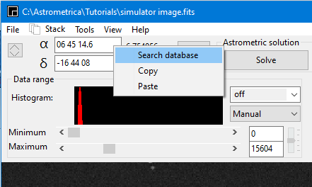
Copy histogram values to clipboard. You can paste them into a spreadsheet.
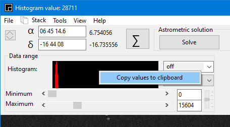
Fits header editor
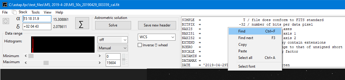
Status bar. You can select to display:
- A different unit for the position.
- The HFD and FWHM in arc seconds.
- Noise reported in electrons.
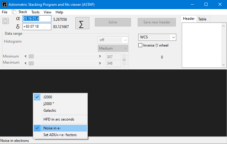
Back to index
Usage as astrometric solver and command line options:
For images in the viewer:
The simplest way to solve an image is just to load an image in the viewer and hit the solve button. Some settings are available in the ∑ menu under tab alignment.
- Diameter field: This is the square size of the star field in degrees used for detection and will be set automatically for most FITS files. It should be in range with the image diameter.
- Radius search: Search radius in degrees. If there is no match, the program will move the search field around in a square spiral and increase the distance from the initial position up to the radius specified. A radius of 30 degrees could be searched in a few minutes.
- Maximum number of stars to use: No need to change it. This could be set between 100 and 1000. Default 500.
- Hash code tolerance: No need to change it. Leave this at 0.007 unless you have severe optical distortion.
- Downsampling: For large image with a height above 3000 pixels select downsampling factor 2 or to speed up the solving and increase the signal noise ratio of the stars. Also colours are combined to monochromatic so this option is beneficial for DSLR images
The solution will be added to the fits header and the centre of the image will be displayed in the log of the ∑ menu. Click on the save button to save the FITS file with the solution. With the solution, the status bar will show the astronomical position of the mouse pointer.
Quick checklist for solving:
- An approximate celestial position is specified (for a spiral search). This position should be displayed in left top left of the viewer menu. (unless you do a 180 degree search)
- Correct image height in degrees specified within preferably 5% accuracy. This height (width x height) should be displayed in the status bar of the viewer and in tab alignment under "Field of view (height)" (Check focal length, sensor size settings or try FOV=auto once)" You can set/force a "Field of view (height)" in tab Alignment.
- At least 30 stars are visible. For small field-of-view (<0.6°) and away from the Milky-Way-plane expose longer up to 30 seconds and install the D20 or D50 star database.
- The stars are reasonably round and the camera is in focus.
- Image dimensions at least 1280x960 pixels. For smaller dimensions solving is still possible if the image quality is good.
- Image is not stretched, very saturated or heavily photo-shopped.
- Try to test if an image is blind solvable.
The internal astrometric solver works best with raw unstretched and sharp images of sufficient resolution where stars can be very faint. Heavily stretched, saturated, out-of-focus or photo shopped images are problematic. It requires a minimum about 30 stars in the image to solve. Images containing a few hundred detectable stars stars are ideal. For star rich images, the program will reduce the detection limit to limit the number of stars. This will only work for unstretched images where brighter stars have a greater intensity than fainter stars. So ASTAP requires three star dimensions for solving. The star x, y coordinates and star intensity to select a subset of the brightest stars. Stars streaks due to tracking errors or severe optical distortion will be ignored and solving could fail.
Check list for successful solving with ASTAP:
- An approximate α and δ celestial position is specified (for a spiral search). For FITS file this position is normally read from the FITS file header and set automatically. The position can also be passed by the command-line from your favourite imaging program. In case you view an JPEG, TIFF image the approximate position can be entered by a double click on α input to search for a known deep sky object position from the database.
- Correct image height in degrees specified within preferably 5% accuracy. See ∑ window, tab alignment, group-box astrometric settings, "Field of view (height)". For FITS images this is normally automatic calculated from info in the file header. In case of doubt you could try "Field of view (height)"=AUTO
- At least 30 stars are visible in the image. They can be very faint, barely visible in the noise. For large field-of-view (>1°) expose 5 to 10 seconds but for small field-of-view (<0.5°) expose longer up to 60 seconds and use the D80 star database.
- The visible stars are reasonable round and the camera is in focus. You could verify the star detection by the CCD inspector or by the Test button to show quads in the ∑ window, tab alignment). Most stars should be detected.
- Image dimensions at least 1280x960 pixels. Set downsample at 0 (=auto) and the program will select a downsampling factor automatically. Image height in pixels after ASTAP dowsampling should be somewhere between 1000 and 3000 pixels. ASI120MC camera image are problemetic to solve.
- Image is not stretched, very saturated or heavily photo-shopped. The total exposure time could be hours (stacked) as long it is possible to separate the brightest stars from the faint by intensity.
- Search radius should be set large enough. See ∑ window, tab alignment, group-box astrometric settings. You could set this at 30° or for blind solving at 180°.
- Use downsample factor 0 (auto). See ∑ window, tab alignment, group-box astrometric settings.
- If your image is full of hot pixels you could adjust the "Ignore stars less than ["]" in tab Alignment. This is set default at 1.5" but could be set higher for a long focal length.
- The maximum number of stars to use should be defined. Typical set at 500. See ∑ window, tab alignment.
- Hash code tolerance should be defined. Typical set at 0.007. See tab alignment.
- For a field-of-view less than 40 arc minutes (long focal length) it is recommend to install the D20, D50 or even the D80 star database. See star database usability
- If a global cluster fills the whole field, ASTAP could struggle to solve. Forcing option "slow" could help.
- Best input format is FITS, RAW or 16 bit PNG, TIFF. Images in 8 bit PNG, TIFF and especially in the JPEG format are disadvantageous for solving.
- If your image has a strong gradient, the option "Equalise background" in tab alignment (or by command-line) could help.
Test if an image is solvable (fully blind solving):
To test if an image is solvable follow this procedure:
A) Load an image in ASTAP
B) Check star detection by hitting button F4. Only stars should be annotated and not the hot pixels. If hot pixels are annotated see E) Hot pixels seen as stars
C) Go to ASTAP settings by CTRL+A or Σ button. Select tab Alignment. Set ASTAP to blind solving by 1) in screen shot below. So "field of view"=auto and "radius of search area[°]"=180. (Note that blind solving will only search within FOV range 10° to 0.3°)
D) Hit the ASTAP
solve button
If too many hot pixels are detected as stars then increase "Ignore stars less than ["]" value marked by 2) in the screen shot. The star annotation values shown after hitting F4 are indicating which value is you should use. More than the hot pixels HFD values but less than the star HFD values. Save settings by hitting the solve button.
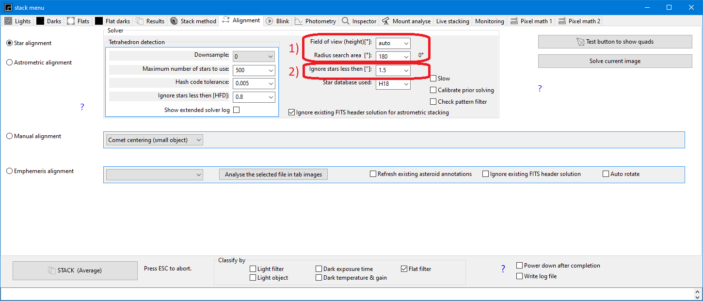
The FOV calculator in tab Pixel math 2
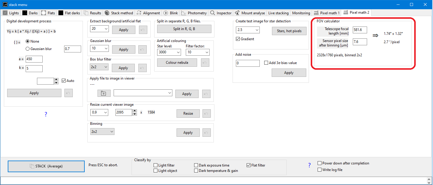
The program can be used to astrometric solve images using the following command line options:
ASTAP astrometric solver command line |
The FOV, RA,DEC parameters are intended for none FITS files. They are not required for FITS files having the values in the header. | ||
|
command
|
parameter | unit | remarks |
| -h | help info | ||
| -help | help info | ||
| Solver options: | |||
| -f | file_name | Image file to solve astrometric. Valid formats FITS, TIFF, PNG, JPG, uncompressed XISF files. | |
| -r | radius_search_field | degrees | The radius of the square search pattern around the start position. * |
| -fov | field_height_of_image | degrees | If not specified it will be extracted from the FITS header or last successful solve will be used (learn mode). Specify 0 for auto. * |
| -ra | right_ascension | hours | If not specified it will be extracted from the FITS header or last successful solve will be used (learn mode). * |
| -spd | south_pole_distance (dec+90) |
degrees | The
declination is given in south
pole distance so always positive. If not specified it will be extracted from the FITS header or last successful solve will be used (learn mode). * |
| -z | down_sample_factor |
0,1,2,3,4,.. | Down sample (binning) of the input image prior to solving. Specify "0" for auto selection.. * |
| -s | max_number_of_stars | Limits the number of star used for the solution. Typical value 500. * | |
| -t | quad_tolerance | ‰ |
Tolerance used to compare quads. Typical value 0.007. * |
| -m | minimum star size | arcsec | This setting could be used to filter out hot pixels. |
| -check | apply | y/n | Apply a check pattern filter prior to solving. Use for raw OSC images only when binning is set 1x1 * |
| -d | path | Specify a path to the star database | |
| -D | abbreviation | d80/d50/... | Specify a star database |
| -o | file | Name the output files with this base path & file name | |
| -sip | add | y/n | Add SIP (Simple Image Polynomial) coefficients. Only required to deactivate SIP. |
| -speed | mode | slow / auto | "slow" is forcing more area overlap while searching to improve detection. * |
| -wcs | Write a .wcs file in similar format as Astrometry.net. Line length fixed at 80 bytes and no carriage returns. Else text style | ||
| -update | Add the solution to the input fits/tiff file header. In case the input is a jpeg, png a new fits will be created. | ||
| -log | Write solver log to a .log text file. | ||
| Analyse options | |||
| -analyse | snr_minimum | Analyse
only and report HFD. Windows: errorlevel is the median HFD * 100M +
number of stars used. So the HFD is trunc(errorlevel/1M)/100. For Linux and macOS the info is send to stdout only. |
|
| -extract | snr_minimum | Export info of all detectable stars to a .csv file. The decimal separator is always a dot. | |
| -extract2 | snr_minimum | Solve
image and export info of all detectable stars to a .csv file
including
α, δ of each detection. SIP polynomial
will be used for high precision positions. The decimal separator
is always a dot. In versions after 2024-2-1 |
|
| * Defaults can be set in the program. Shortcut CTRL-A, tab alignment | |||
| Extra options below are only for the standard GUI version of ASTAP. Not for the ASTAP_CLI command-line version. | |||
| -annotate | Produce a deep sky annotated jpeg file with same name as input file extended with _annotated. | ||
| -debug | Show GUI and stop prior to solving | ||
| -tofits | binning | 1,2,3,4 | Produce binned FITS file from input png/jpg |
| As analyser/stacker: | |||
| -sqm | pedestal | Measure the sky background value in magn/arcsec2 relative to the stars. The pedestal is the mean value of a dark. Also centalt and airmass are written to the header.. | |
| -focus1 | file1.fits -focus2 file2.fits -focus3 file3.fits ................ | Find best focus point for four or more images using curve fitting. Windows: errorlevel is focuspos*1E4 + rem.error*1E3. Linux: see stdout | |
| -stack | path | Start ASTAP with live stack tab visible and path selected. | |
| -p | path | Create a photometry report of the files in the path. Settings should come from an .ini file in the same path | |
Command-line parameters have priority above fits header values. Front-end programs should provide access to -z and -r options as a minimum. Default value for -z should be 0 (auto).
Typical command lines:
astap.exe -f image.fits -r 50
astap.exe -f c:\images\image.png -ra 23.000 -spd 179.000 -fov 1.3 -r 50
For most FITS files the command line can be short since telescope position and field of view can be retrieved from the FITS header. The keywords read are documented in appendix 4 FITS keywords read for solving. If a FITS file is not available, preference is a non lossless image format like .PNG or .TIFF or RAW like .CR2. If possible in 16 bit or original 12 bit format. Not stretched or saturated, as raw as possible. For formats other then FITS the RA,DEC position and -fov (image HEIGHT in degrees !!) should be added.
If the FOV (image height in degrees) is unspecified in the command-line for RAW, PNG, TIFF files, ASTAP will use the FOV as set in the program, stack menu, tab alignment. This setting can be learned and updated automatically with the parameters -fov 0. ASTAP will try all FOV between 10 degrees and 0.3 degrees. E.g.
astap.exe -f c:\images\image.png -ra 23.000 -spd 179.000 -r 30 -fov 0
After a successful solve, the correct FOV will be stored in the ASTAP settings. For the next solve using images from the same source the -fov 0 parameters can be omitted and solving will be fast.
The
debug option allows to set some solving parameters in the GUI
(graphical user interface) and to test the commandline. In debug mode
all commandline parameters are set and the specified image is shown in
the viewer. Only the solve command has to be given manually:
astap.exe -f c:\images\image.png -ra 23.000 -spd 179.000 -r 30 -debug
or
astap.exe -debug
Command-line, output files
In command line mode the program produces two output files at the same location as the input image. In case a solution is found it will write a .wcs file 1) containing the solved FITS header only. In any case it will write an INI file using the standard FITS keywords.
PLTSOLVD=T
// T=true, F=false
CRPIX1= 1.1645000000000000E+003
// X of
reference & centre pixel
CRPIX2=
8.8050000000000000E+002
// Y of
reference & centre pixel
CRVAL1= 1.5463033992314939E+002
// RA (J2000) of the reference pixel
[deg]
CRVAL2=
2.2039358425145043E+001
// DEC (J2000)of the reference pixel
[deg]
CDELT1=-7.4798001762187193E-004
// X pixel
size [deg]
CDELT2=
7.4845252983311850E-004
// Y pixel
size [deg]
CROTA1=-1.1668387329628058E+000
// Image
twist of X axis [deg]
CROTA2=-1.1900321176194073E+000
// Image
twist of Y axis [deg]
CD1_1=-7.4781868711882519E-004
// CD
matrix to convert (x,y) to (Ra, Dec)
CD1_2= 1.5241315209850368E-005
// CD
matrix to convert (x,y) to (Ra, Dec)
CD2_1= 1.5534412042060001E-005
// CD
matrix to convert (x,y) to (Ra, Dec)
CD2_2= 7.4829732842251226E-004
// CD matrix to convert (x,y) to (Ra, Dec)
CMDLINE=......
// Text message containing command
line used
WARNING=......
// Text message containing
warning(s)
PLTSOLVD=F
// T=true, F=false
CMDLINE=......
// Text message containing command
line used
ERROR=
.....
// Text message
containing any error(s). Same as exit code errors
WARNING= .....
// Text
message containing any warnings(s)
The .wcs file contains the original FITS header with the solution added. No data, just the header. Any warning is added to the .wcs file using the keyword WARNING. This warning could be presented to the user for information.
1) Note the wcs file is default written as text file using carriage return and line feed for each line and is not conform the FITS standard. To have .wcs file conform the FITS standard add the command-line option -wcs.
Command-line, error codes
In the command-line mode errors are reported by an error code / errorlevel {%errorlevel%}. This is the same error as reported in the .ini file in case of failure.
| Error code | Description |
| 0 | No errors |
| 1 | No solution |
| 2 | Not enough stars detected |
| 16 | Error reading image file |
| 32 | No star database found |
| 33 | Error reading star database |
| 34 | Error updating input file |
c:\astap.fpc\astap.exe -f c:\astap.fpc\test_files\command_line_test\m16.fit -analyse 30
echo Exit Code is %errorlevel%
pause
You will get
Exit Code is 326000666
where the HFD is 3.26 using 666 stars
For Linux and Mac a stdout is used reporting as follows:
HFD_MEDIAN=3.3
| Program | Windows | Linux | macOS |
| astap | exit code | stdout | stdout |
| astap_cli | exit code & stdout | stdout | stdout |
Finding best focus based on four or more input images:
c:\astap.fpc\astap -focus1 D:\temp\FocusSample\FOCUS04689.fit -focus2 D:\temp\FocusSample\FOCUS05039.fit -focus3 D:\temp\FocusSample\FOCUS05389.fit -focus4 D:\temp\FocusSample\FOCUS05739.fit -focus5 D:\temp\FocusSample\FOCUS06089.fit -focus6 D:\temp\FocusSample\FOCUS06439.fit -focus7 D:\temp\FocusSample\FOCUS06789.fit -focus8 D:\temp\FocusSample\FOCUS07139.fit
echo Exit Code is %errorlevel%
pause
or with the -debug option
astap.exe -debug -focus1 D:\temp\FocusSample\FOCUS04689.fit -focus2 D:\temp\FocusSample\FOCUS05039.fit -focus3 D:\temp\FocusSample\FOCUS05389.fit -focus4 D:\temp\FocusSample\FOCUS05739.fit -focus5 D:\temp\FocusSample\FOCUS06089.fit -focus6 D:\temp\FocusSample\FOCUS06439.fit -focus7 D:\temp\FocusSample\FOCUS06789.fit -focus8 D:\temp\FocusSample\FOCUS07139.fit
Select then tab "inspector" and hit the "hyperbola curve fitting button" to test the functionality.
Here an example of the command-line output: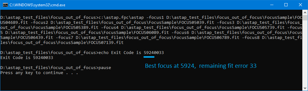
This option is not available for the astap_cli version.
If the ASTAP is command-line executed in MS-Windows, it will be shown by a small ASTAP tray icon on the right side of the status bar. If you move the mouse to the ASTAP tray icon, the hint will show the search radius reached. To refresh the value move the mouse away and back.
If the search spiral has reached a distance more than 2 degrees from the start position then a pop-up notifier will show the actual search distance and solver settings:
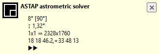
- The first line indicates the search spiral distance (8º) from the start position and the maximum search radius (90º)
- The image height in degrees.
- Downsample setting and the input dimensions of the image to solve.
- The α and δ of the start position.
- Speed normal (▶▶) or small steps (▶)
Tray icons are default off in the latest Win10 version. To set the ASTAP tray icon on, start a solve via the imaging program, go to Windows "Settings", "Taskbar", "Turn system icons on or off" and set the ASTAP tray icon permanent "on" as shown below:
![]()
Blind solving performance for a 90 degrees offset:
| ASTAP blind solver performance
for a 90 degrees offset. Solving a 50 seconds exposed monochrome image of M16, 2328x1760 pixels covering a field of 1.75 x 1.32° starting 90 degrees more north. Database used D50 |
|
| Maximum stars set | Astrometric solving time |
| 500 | 23.8 sec. |
| 300 | 9.8 sec |
| 200 | 6.7 sec |
| 100 | 4.8 sec |
| Reducing the "maximum number of stars to use" will result in a faster solving but also an increased risk of solve failure. | |
Installation of the external Astrometry.net solver:
MS-Windows:
Install a local copy
of Astrometry.net (via ANSVR or Astrotortilla)
as the astrometric
solver. Or alternatively if you have Win10, 64 bit Creation
edition you use the new Linux sub-system
ANSVR: The ANSVR link contains a newer compilation of astrometry.net made for SGP. It runs as a Linux program under Cygwin in MSWindows. Follow up to installation step 9. The link you have to put in ASTAP is as follows:
C:\Users\user_name\AppData\Local\cygwin_ansvr\bin\bash.exe
Adapt "user_name" to the login name used in Windows.
The server program ANSVR is not required. Remove the ANSVR shortcut in the startup menu. Location:
C:\Users\user_name\AppData\Roaming\Microsoft\Windows\Start Menu\Programs\Startup
Alternative Linux sub-system in Win10 64bit Creators edition
Path for the astrometry.net solver program
ANSVR installation:
C:\Users\user_name\AppData\Local\cygwin_ansvr\bin\bash.exe
Astrotortilla installation:
C:\cygwin\bin\bash.exe
Win10 subsystem:
C:\Windows\System32\bash.exe
If you want to use astrometry.net this is described at installation. To get the Astrometry.net solver type: sudo apt-get install libcairo2-dev libnetpbm10-dev netpbm libpng-dev libjpeg-dev python-numpy python-pyfits python-dev zlib1g-dev libbz2-dev swig libcfitsio-dev You also have to download index files.
Path to the astrometry.net solver program "solve-field" could be:
/usr/bin/
or
/usr/local/astrometry/bin
The master flat is calculated as:
master flat: = (1/n ∑ [flats] - 1/n ∑ [flat darks] )
Where a bias image could be used as flat-dark image. The master flat should be averaged by a 2x2mean to remove Bayer matrix artifacts.
Each image is calculated as:
(image- {1/n∑ [darks]} ) / master flat
Then the Bayer matrix is applied and finally the images are stacked in mode average or sigma clipped.
So for average stack:
final image:= 1/n ∑ Bayer(image)
The main reason why you have to use flat-darks or bias frames is that they provide a pedestal so a fixed value to the flat routine. The same pedestal value which is present in the flat. This is typical a pixel value of something around 500 to 1000. Without this value the flat compensation will not work properly, and the darker corners of the light frame(s) will be under compensated.
This can be visualised with a simple X, Y diagram. The green part of the value is due to the light exposure. Blue is the pedestal value. If the flat-dark is included (subtracted) the intensity at the corners of the sensor drops to 40000/50000 equals 80%. If no flat-dark is included, then the measured intensity drop will be 41000/51000 equals 80.3%. This will result in an under compensation by the flat routine and the corners of the stack will be a little darker than the centre. So use flat-darks or bias frames for best flat correction.
Some cameras behave a little weird in the first second. For those it could be better to use the same exposure time for the flat-dark as for the flat. A bias is a flat-dark with an exposure time 0 or about zero. For most cameras you will not notice the difference between using either a bias or flat-dark.
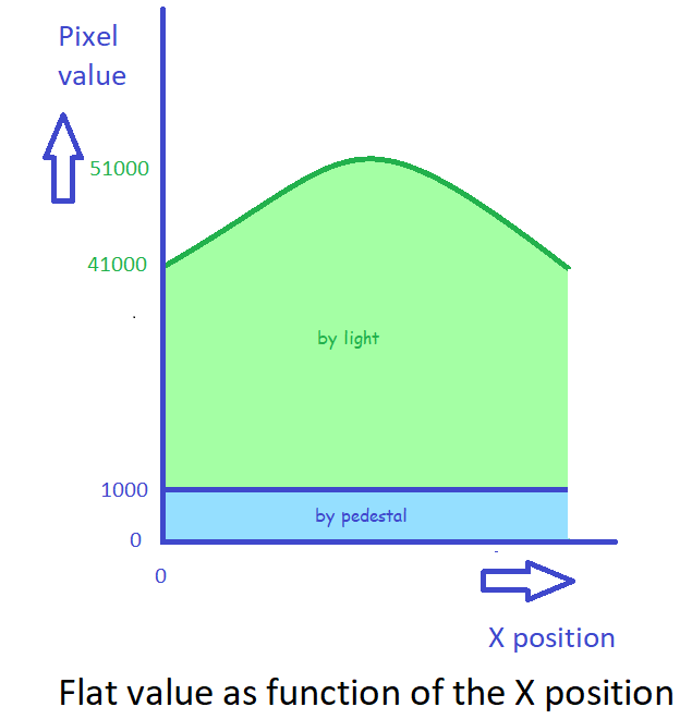
The dark temperature should be about equal as the the light temperature. Calibration with a master dark of a lower temperature gives a poorer result than calibration with a master dark of equal temperature. See test results below:
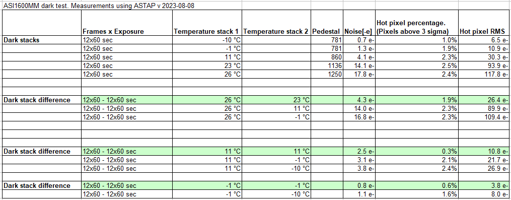
Appendix 3, the 1476 and 001 star database format:
The 1476 format:
The .1476 format divides the sky in 1476 area's and 1476 corresponding files with the extension .1476. The 1476 areas have a minimum width or diameter of 90°/17.5 equals 5.143°. The boundaries are defined by constant α and δ values. For the similar 290 file format see the HNSKY help file
Each star is stored in a record of 5 bytes. The files start 'with a 110 byte header containing a textual description and the record size binary stored in byte 110. The RA values are stored as a 3 bytes word. The DEC positions are stored as a two's complement (=standard), three bytes integer. The resolution of this three byte storage will be for RA: 360*60*60/((256*256*256)-1) = 0.077 arc seconds. For the DEC value it will be: 90*60*60/((128*256*256)-1) = 0.039 arc seconds. The stars are sorted on magnitude and the magnitude is stored in a byte of the special preceding header with an offset to make all values positive.
Example of star Sirius RA and DEC position:
The RA position is stored as C3 06 48 equals: (195 +6*256 +72*256*256)*24/((256*256*256)-1)=6.75247662 hours equals: 6:45:8.9
The DEC position is stored as D7 39 E8, equals: 215 57 -24. The DEC is then (215 +57*256 -24*256*256)*90/((128*256*256)-1)=-16.7161401 degrees equals -16d 42 58
Record format:
The 1476-5 or 290-5, short record size of 5 bytes for one star without designation used for the G05, D05, D20,D50:
type
hnskyhdr1476 = packed record
ra7 : byte;
ra8 : byte;
ra9 : byte;
dec7 : byte;
dec8 : byte;{magnitude and dec9 are written once in preceding header-record}
end;
The 1476-6 or 290-6, short record size of 6 bytes for one star without designation: used for the V50
type
hnskyhdr1476 = packed record
ra7 : byte;
ra8 : byte;
ra9 : byte;
dec7 : byte;
dec8 : byte;{magnitude and dec9 are written once in preceding header-record}
B_R : shortint;{Gaia Bp-Rp}
end;
Stars are sorted from bright to faint in the "0.1" steps. Within the magnitude range, the stars are additional sorted in DEC. For a series of stars with the same DEC9 value, a header-record is preceding containing the DEC9 value stored at location DEC7. Since the stars are already sorted in 36 declination bands, the number of DEC9 values is already limited by a factor 36.
1476-5 header-record example: FF FF FF 20 06 This indicates the following records have a DEC9 value of 20 -128 offset and a magnitude of (06 - 16)/10 equals -1.0 (new method, +16 offset).
The shorter records methods become only space efficient for very large star collection of a few million stars. In these large collections many stars can be found with the same magnitude and DEC9 shortint. The Gaia database is issued in the 1476-5 format of 5 bytes per star or 1476-6 of 6 bytes per star (V50). An older format 290-5 is used for larger field of view (G05. Thes 290 areas are documented in the HNSKY planetarium program help file.
So the record sequence will be as follows:
record
record
record
record
header-record {new section will start with a different magnitude and dec9}
record
record
The 1476 areas: Each ring is divided by lines of constant RA such that the minimum width in RA is about 5 degrees (deltaRA*cos(DEC)
.
| Declination minimum | Declination maximum | Ring | RA cells | RA step north[degr] | RA step distance south[degr] | DEC step | Files | |
| -90.00000000 | -87.42857143 | 0-1 | 1 | 0101.1476 | ||||
| -87.42857143 | -82.28571429 | 1-2 | 3 | 5.38377964 | 16.10799190 | -2.57142857 | {=90/(2*17.5)} | 0201.1476, 0202.1476, 0203.1476 |
| -82.28571429 | -77.14285714 | 2-3 | 9 | 5.36933063 | 8.90083736 | -5.14285714 | {=90/17.5} | 0301.1476, . . . . . , 0309.1476 |
| -77.14285714 | -72.00000000 | 3-4 | 15 | 5.34050241 | 7.41640786 | -5.14285714 | {=90/17.5} | 0401.1476, . . . . . , 0415.1476 |
| -72.00000000 | -66.85714286 | 4-5 | 21 | 5.29743419 | 6.73757197 | -5.14285714 | 0501.1476, . . . . . , 0521.1476 | |
| -66.85714286 | -61.71428571 | 5-6 | 27 | 5.24033376 | 6.31824883 | -5.14285714 | 06 . . . | |
| -61.71428571 | -56.57142857 | 6-7 | 33 | 5.16947632 | 6.00978525 | -5.14285714 | 07 . . . | |
| -56.57142857 | -51.42857143 | 7-8 | 38 | 5.21902403 | 5.90674549 | -5.14285714 | 08 . . . | |
| -51.42857143 | -46.28571429 | 8-9 | 43 | 5.21991462 | 5.78564078 | -5.14285714 | 09 . . . | |
| -46.28571429 | -41.14285714 | 9-10 | 48 | 5.18296987 | 5.64803600 | -5.14285714 | 10 . . . | |
| -41.14285714 | -36.00000000 | 10-11 | 52 | 5.21357169 | 5.60088688 | -5.14285714 | 11 . . . | |
| -36.00000000 | -30.85714286 | 11-12 | 56 | 5.20082354 | 5.51859939 | -5.14285714 | 12 . . . | |
| -30.85714286 | -25.71428571 | 12-13 | 60 | 5.15069276 | 5.40581321 | -5.14285714 | 13 . . . | |
| -25.71428571 | -20.57142857 | 13-14 | 63 | 5.14839353 | 5.34991355 | -5.14285714 | 14 . . . | |
| -20.57142857 | -15.42857143 | 14-15 | 65 | 5.18530082 | 5.33887123 | -5.14285714 | 15 . . . | |
| -15.42857143 | -10.28571429 | 15-16 | 67 | 5.17950194 | 5.28678585 | -5.14285714 | 16 . . . | |
| -10.28571429 | -5.14285714 | 16-17 | 68 | 5.20903900 | 5.27280509 | -5.14285714 | 17 . . . | |
| -5.14285714 | 0.00000000 | 17-18 | 69 | 5.19638762 | 5.21739130 | -5.14285714 | 18 . . . | |
| 0.00000000 | 5.14285714 | 18-19 | 69 | 5.21739130 | 5.19638762 | -5.14285714 | 19 . . . | |
| 5.14285714 | 10.28571429 | 19-20 | 68 | 5.27280509 | 5.20903900 | -5.14285714 | 20 . . . | |
| 10.28571429 | 15.42857143 | 20-21 | 67 | 5.28678585 | 5.17950194 | -5.14285714 | 21 . . . | |
| 15.42857143 | 20.57142857 | 21-22 | 65 | 5.33887123 | 5.18530082 | -5.14285714 | 22 . . . | |
| 20.57142857 | 25.71428571 | 22-23 | 63 | 5.34991355 | 5.14839353 | -5.14285714 | 23 . . . | |
| 25.71428571 | 30.85714286 | 23-24 | 60 | 5.40581321 | 5.15069276 | -5.14285714 | 24 . . . | |
| 30.85714286 | 36.00000000 | 24-25 | 56 | 5.51859939 | 5.20082354 | -5.14285714 | 25 . . . | |
| 36.00000000 | 41.14285714 | 25-26 | 52 | 5.60088688 | 5.21357169 | -5.14285714 | 26 . . . | |
| 41.14285714 | 46.28571429 | 26-27 | 48 | 5.64803600 | 5.18296987 | -5.14285714 | 27 . . . | |
| 46.28571429 | 51.42857143 | 27-28 | 43 | 5.78564078 | 5.21991462 | -5.14285714 | 28 . . . | |
| 51.42857143 | 56.57142857 | 28-29 | 38 | 5.90674549 | 5.21902403 | -5.14285714 | 29 . . . | |
| 56.57142857 | 61.71428571 | 29-30 | 33 | 6.00978525 | 5.16947632 | -5.14285714 | 30 . . . | |
| 61.71428571 | 66.85714286 | 30-31 | 27 | 6.31824883 | 5.24033376 | -5.14285714 | 31 . . . | |
| 66.85714286 | 72.00000000 | 31-32 | 21 | 6.73757197 | 5.29743419 | -5.14285714 | 32 . . . | |
| 72.00000000 | 77.14285714 | 32-33 | 15 | 7.41640786 | 5.34050241 | -5.14285714 | 33 . . . | |
| 77.14285714 | 82.28571429 | 33-34 | 9 | 8.90083736 | 5.36933063 | -5.14285714 | 34 . . . | |
| 82.28571429 | 87.42857143 | 34-35 | 3 | 16.10799190 | 5.38377964 | -5.14285714 | 3501.1476, 3502.1476, 3503.1476 | |
| 87.42857143 | 90.00000000 | 36-37 | 1 | 3601.1476 |
The 1476 areas:
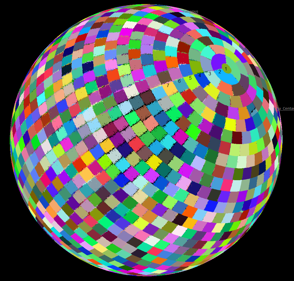
South pole view of the 1476 areas:
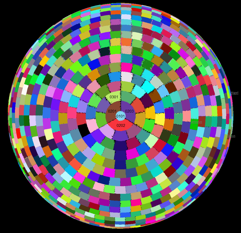
The 001 format:
For wide field the stars are stored in a single file w08.001 down to magnitude 8. The stars are sorted from bright to faint. The file starts with a 4 byte integer specifying the number of records=stars and has for the W08 value 41246. Each star is stored in a record of three singles (4 byte floats). Starting with magnitude [x10] then RA [radians] and finally DEC[radians]. So the data is written as the following array (first star is Sirius):
star_array : array[0..41264,0..2] of single = //all stars up to magnitude 8
(
( -15 , 1.767725252 , -0.291899504 ),
( -6 , 1.675309906 , -0.919709903 ),
( 0 , 4.873596766 , 0.676937966 ),
( 0 , 3.837100429 , -1.061694783 ),
( 0 , 3.73338603 , 0.334553937 ),
( 1 , 1.381830995 , 0.802764629 ),
( 3 , 1.372430608 , -0.143145706 ),
( 4 , 2.003995701 , 0.091067934 ),
Appendix 4, FITS header keywords read for solving
The following FITS header keywords are read to determine the initial celestial position for the solver search and the field of view:
| Celestial position | Keyword | Unit | Description | Source |
| RA | degrees or hh:mm:ss | Telescope pointing RA | input | |
| DEC | degrees or dd:mm:ss | Telescope pointing DEC | input | |
| OBJCTRA | hh:mm:ss | RA of object being imaged | input | |
| OBJCTDEC | dd:mm:ss | DEC of object being imaged | input | |
| CRVAL1 | degrees | RA of reference pixel | solver output | |
| CRVAL2 | degrees | DEC of reference pixel | solver output | |
| Field of view | SECPIX1 | arcsec/pixel | X pixel size | input |
| SECPIX2 | arcsec/pixel | Y pixel size | input | |
| SCALE | arcsec/pixel | Pixel size | input | |
| PIXSCALE | arcsec/pixel | Pixel size | input | |
| FOCALLEN | meter | input | ||
| XPIXSZ | μm | X pixel scale in microns. Includes binning. | input | |
| YPIXSZ | μm | Y pixel scale in microns. Includes binning. | input | |
| CDELT1 | deg/pixel | X pixel size | solver output | |
| CDELT2 | deg/pixel | Y pixel size | solver output | |
| CD keywords | deg/pixel | The four solution keywords | solver output |
Back to index
SIP polynomial coefficients:
The ASTAP solver can add 3th order SIP polynomial coefficients to the header to cope with image distortion.
Adding SIP coefficients ensures accurate positional information of celestial objects and to facilitate precise image stitching. Astronomical images often suffer from barrel distortion, where stars near the edges appear to move outward from the centre of the image. SIP (Simple Image Polynomial) coefficients provide a polynomial model to represent this distortion. This model mathematically describes how the actual positions of stars (or other celestial objects) in the image deviate from their ideal positions on a distortion-free plane. The SIP correction can be tested with the option "Show distortion". The SIP option can be set in the tab alignment and can also be activated by a command-line parameter. The astap_cli command-line version can also add SIP coefficients.
External link:
Developer information: Using SIP Coefficients for optical distortion correction